7.2. Fraud Detection with Python (Github Trenton McKinney)
The notes are based off of McKinney, T. (2019, July 19). Fraud Detection with Python. Fraud Detection with Python - GitHub (Using Jupyter Book): https://trenton3983.github.io/files/projects/2019-07-19_fraud_detection_python/2019-07-19_fraud_detection_python.html.
7.2.1. Background
Fraud is intentional deception with the aim of providing the perpetrator with some gain or to deny the rights of a victim. There are a few models to detect fraud in datasets that we will be going over here.Fraud is intentional deception with the aim of providing the perpetrator with some gain or to deny the rights of a victim. There are a few models to detect fraud in datasets that we will be going over here.
7.2.2. Setting Up Working Enviroment
First we will be importing what will be used in these notes. The packages imblearn and gensim are not by default installed with anaconda and will need to be installed with pip install imblearn, gensim, and nltk. We will also set our configuration options for Pandas at this time.
7.2.2.1. Installation Process
import warnings
warnings.filterwarnings('ignore')
warnings.simplefilter('ignore')
Installing necessary pacakges using !pip3 install using Jupyter Notebook. Commenting out the installation process.
#!pip3 install matplotlib
#!pip3 install gensim
#!pip3 install imblearn
#!pip3 install nltk
#!pip3 install pyldavis
#!pip3 install wget
7.2.2.2. Importing
Importing necessary packages
import pandas as pd
import matplotlib.pyplot as plt
from matplotlib.patches import Rectangle
import numpy as np
from pprint import pprint as pp
import csv
from pathlib import Path
import seaborn as sns
from itertools import product
import string

import nltk
from nltk.corpus import stopwords
from nltk.stem.wordnet import WordNetLemmatizer

from imblearn.over_sampling import SMOTE
from imblearn.over_sampling import BorderlineSMOTE
from imblearn.pipeline import Pipeline

from sklearn.linear_model import LinearRegression, LogisticRegression
from sklearn.model_selection import train_test_split, GridSearchCV
from sklearn.tree import DecisionTreeClassifier
from sklearn.metrics import r2_score, classification_report, confusion_matrix
from sklearn.metrics import accuracy_score, roc_auc_score, roc_curve
from sklearn.metrics import average_precision_score, precision_recall_curve
from sklearn.metrics import homogeneity_score, silhouette_score
from sklearn.ensemble import RandomForestClassifier, VotingClassifier
from sklearn.preprocessing import MinMaxScaler
from sklearn.cluster import MiniBatchKMeans, DBSCAN

import gensim
from gensim import corpora

import wget # helps with installation
import zipfile
import os
import shutil
7.2.2.3. Pandas Configuration Options
pd.set_option('display.max_columns', 700)
pd.set_option('display.max_rows', 400)
pd.set_option('display.min_rows', 10)
pd.set_option('display.expand_frame_repr', True)
7.2.2.4. Data File Objects
We are going to need some data to check for fraud. This chunk of code will download and unpack the data we will be using.
if not os.path.exists("chapter_1.zip"):
    wget.download("https://assets.datacamp.com/production/repositories/2162/datasets/cc3a36b722c0806e4a7df2634e345975a0724958/chapter_1.zip")

if not os.path.exists("chapter_2.zip"):
    wget.download("https://assets.datacamp.com/production/repositories/2162/datasets/4fb6199be9b89626dcd6b36c235cbf60cf4c1631/chapter_2.zip")

if not os.path.exists("chapter_3.zip"):
    wget.download("https://assets.datacamp.com/production/repositories/2162/datasets/08cfcd4158b3a758e72e9bd077a9e44fec9f773b/chapter_3.zip")

if not os.path.exists("chapter_4.zip"):
    wget.download("https://assets.datacamp.com/production/repositories/2162/datasets/94f2356652dc9ea8f0654b5e9c29645115b6e77f/chapter_4.zip")

if not os.path.exists("data/chapter_1"):
    with zipfile.ZipFile("chapter_1.zip", 'r') as zip_ref:
        zip_ref.extractall("data")
    os.remove("chapter_1.zip")

if not os.path.exists("data/chapter_2"):
    with zipfile.ZipFile("chapter_2.zip", 'r') as zip_ref:
        zip_ref.extractall("data")
    os.remove("chapter_2.zip")

if not os.path.exists("data/chapter_3"):
    with zipfile.ZipFile("chapter_3.zip", 'r') as zip_ref:
        zip_ref.extractall("data")
    os.remove("chapter_3.zip")

if not os.path.exists("data/chapter_4"):
    with zipfile.ZipFile("chapter_4.zip", 'r') as zip_ref:
        zip_ref.extractall("data")
    os.remove("chapter_4.zip")

#!unzip chapter_1.zip
#!unzip chapter_2.zip
#!unzip chapter_3.zip
#!unzip chapter_4.zip
data = Path.cwd() / 'data'


ch1 = data / 'chapter_1'
cc1_file = ch1 / 'creditcard_sampledata.csv'
cc3_file = ch1 / 'creditcard_sampledata_3.csv'

ch2 = data / 'chapter_2'
cc2_file = ch2 / 'creditcard_sampledata_2.csv'

ch3 = data / 'chapter_3'
banksim_file = ch3 / 'banksim.csv'
banksim_adj_file = ch3 / 'banksim_adj.csv'
db_full_file = ch3 / 'db_full.pickle'
labels_file = ch3 / 'labels.pickle'
labels_full_file = ch3 / 'labels_full.pickle'
x_scaled_file = ch3 / 'x_scaled.pickle'
x_scaled_full_file = ch3 / 'x_scaled_full.pickle'

ch4 = data / 'chapter_4'
enron_emails_clean_file = ch4 / 'enron_emails_clean.csv'
cleantext_file = ch4 / 'cleantext.pickle'
corpus_file = ch4 / 'corpus.pickle'
dict_file = ch4 / 'dict.pickle'
ldamodel_file = ch4 / 'ldamodel.pickle'
7.2.3. Preparing the Data
Fraud occurs only in an extreme minority of transactions. However, machine learning algorithms learn best when the cases they are looking at are fairly even. Without many datapoints of actual fraud, it is difficult to teach it how to detect fraud. This is called a class imbalance.
Lets start by taking the 'creditcard_sampledata.csv' file and converting it into a Pandas DataFrame and looking at the the DataFrame so we know what we’re working with.
df = pd.read_csv(cc3_file) # Create Pandas DataFrame from our file

df.info() # Gives information on the type of data in the DataFrame

df.head() # Shows the first few rows of the DataFrame
7.2.3.1. Visualizing the Fraudulent data
Here, the fraudulent status of the data is already known in the Class column (0 is non-fraudulent, 1 is fraudulent). The data in columns V1-V28 are about the transactions for each account. Lets take a look at how many fraudulent cases there are and what the ratio of fraudulent to non-fraudulent cases is.
# Counts the number of fraud and no fraud occurances
occ = df['Class'].value_counts()
occ
# Prints the ratio of fraud to non-fraud cases
ratio_cases = occ/len(df.index)
print(f'Ratio of fraudulent cases: {ratio_cases[1]}\nRatio of non-fraudulent cases: {ratio_cases[0]}')
See how low the ratio of fraudulent cases is! This is what we need to deal with.
Let’s now plot the fraudulent and non-fraudulent data so we get a better idea of what we are working with. Lets define two functions: prep_data() and plot_data(). The first will take in our original DataFrame and return X and y DataFrames only containing the transaction data and if the account is fraudulent respectively. The second will take our data from prep_data() and plot the V2 vs V3 values coloring them by if they are fraudulent.
def prep_data(df: pd.DataFrame) -> (np.ndarray, np.ndarray):
    """
    Convert the DataFrame into two variable
    X: data columns (V2 - Amount)
    y: lable column
    """
    X = df.iloc[:, 2:30].values
    y = df.Class.values
    return X, y

# Define a function to create a scatter plot of our data and labels with x being V2 and y being V3
def plot_data(X: np.ndarray, y: np.ndarray):
    plt.scatter(X[y == 0, 0], X[y == 0, 1],
                label = "Class #0", alpha = 0.5, linewidth = 0.15)
    plt.scatter(X[y == 1, 0], X[y == 1, 1],
                label = "Class #1", alpha = 0.5, linewidth = 0.15, c = 'r')
    plt.xlabel("V2")
    plt.ylabel("V3")
    plt.legend()
    return plt.show()
# Create X and y from the prep_data function
X, y = prep_data(df)

# Plot our data by running our plot data function on X and y
plot_data(X, y)
7.2.3.2. Data Resampling
We can resample our data to better account for the imbalance in the dataset. This can be done by Undersampling or Oversampling. To be able to compare the resampled datasets let us define a compare_plot() function which will take in two DataFrames and return a comparison of the two plots.
def compare_plot(X: np.ndarray, y: np.ndarray, X_resampled: np.ndarray, y_resampled: np.ndarray, method: str):
    plt.subplot(1, 2, 1)
    plt.scatter(X[y == 0, 0], X[y == 0, 1],
                label = "Class #0", alpha = 0.5, linewidth = 0.15)
    plt.scatter(X[y == 1, 0], X[y == 1, 1],
                label = "Class #1", alpha = 0.5, linewidth = 0.15, c = 'r')
    plt.xlabel("V2")
    plt.ylabel("V3")
    plt.title('Original Set')
    plt.subplot(1, 2, 2)
    plt.scatter(X_resampled[y_resampled == 0, 0],
                X_resampled[y_resampled == 0, 1],
                label = "Class #0", alpha = 0.5, linewidth = 0.15)
    plt.scatter(X_resampled[y_resampled == 1, 0],
                X_resampled[y_resampled == 1, 1],
                label = "Class #1", alpha = 0.5, linewidth = 0.15, c = 'r')
    plt.xlabel("V2")
    plt.title(method)
    plt.legend()
    plt.show()
7.2.3.2.1. Undersampling
Straightforward method that randomly samples our majority (non-fraudulent) cases to get a new set which is about equal to our minority (fraudulent) data. This can be convenient if there is a lot of data with a great deal of minority cases, however usually we do not want to throw away data.
7.2.3.2.2. Random Oversampling
Oversampling involves somehow creating more minority (fraudulent) data. The most straightforward method involves randomly duplicating the minority (fraudulent) datapoints. There is a function in imblearn which can do this. This trains the model on duplicates and isn’t always ideal. You can tell the points are duplicated in the comparison plot because they are darker, having multiple points on the same location.
from imblearn.over_sampling import RandomOverSampler

method = RandomOverSampler()
X_resampled, y_resampled =  method.fit_resample(X, y)

compare_plot(X, y, X_resampled, y_resampled,
             method = "RandomOverSampling")
7.2.3.2.3. Synthetic Minority Oversampling Technique (SMOTE)
SMOTE is a technique which attempts to rectify imbalances by using the characteristics of neighbor minority data to create synthetic fraud cases. This avoids duplicating any data, is fairly realistic, but only works if the minority cases have similar features.
# Run the prep_data function
X, y = prep_data(df)

# Define the resampling method
method = SMOTE()

# Create the resampled data set
X_resampled, y_resampled = method.fit_resample(X, y)
# Show the number of datapoints for non-fraudulent and fraudulent cases in the original data
pd.value_counts(pd.Series(y))
# Show the number of datapoints for non-fraudulent and fraudulent cases in the resampled data
pd.value_counts(pd.Series(y_resampled))
compare_plot(X, y, X_resampled, y_resampled, method = 'SMOTE')
7.2.4. Applying Fraud Detection Algorithms
Generally there are two types of systems for detecting fraud: Rules Based and Machine Learning (ML) Based.
Rules based uses a set of rules to catch fraud such as transactions occurring at odd zipcodes or too frequent transactions. This can catch fraud but also generates a lot of false positives. In addition they do not adapt over time, are limited to yes/no outcomes, and fail to recognize possible interactions between features.
ML based adapt to data, using all the combined data to deliver a probability a transaction is fraudulent. This works much better and can be combined with a rules based approach.
7.2.4.1. Traditional Fraud Detection
Traditional fraud detection involves defining threshold values using common statistics for split fraud and non-fraud data, then use those thresholds to detect fraud. This is often done by looking at the means for differences.
First we will clean up the data slightly and use Pandas .groupby() and .mean() functions to find the means of each column of interest split up by non-fraud and fraud cases. We can then look at this to create a rule which might catch fraud cases.
df.drop(['Unnamed: 0'], axis = 1, inplace = True)
df.groupby('Class').mean()
It looks like fraud cases have V1 < -3 and V3 < -5, so lets implement that as a rule. We will add a new column called flag_as_fraud and place a 1 where that rule is true and 0 where it is false using numpy.where(). We will compare this to if there is a case of actual fraud using pandas.crossttab().
df['flag_as_fraud'] = np.where(np.logical_and(df.V1 < -3, df.V3 < -5), 1, 0)
pd.crosstab(df.Class, df.flag_as_fraud,
            rownames = ['Actual Fraud'], colnames = ['Flagged Fraud'])
With this rule 22/50 of fraud cases were detected, 28/50 were not detected, and there were 16 false positives. Not ideal!
7.2.4.2. Using ML Classification - Logistic Regression
Lets use machine learning on our credit card data instead by implementing a Logistic Regression model.
When fitting models there are a few things to keep in mind. The data should be first split into test and train data using functions such as sklearn.model_selection.train_test_split(). Then only the training data should be resampled. The model is then fitted to the resampled data. Then the results predicted from the model are to be compared using functions such as sklearn.metrics.classification_report() and sklearn.metrics.confusion_matrix().
# Create the training and testing sets, with 30% of the data used for our test data.
X_train, X_test, y_train, y_test = train_test_split(X, y, test_size = 0.3, random_state = 0)

# Fit a logistic regression model to our data
model = LogisticRegression(solver = 'liblinear')
model.fit(X_train, y_train)

# Obtain model predictions
predicted = model.predict(X_test)

# Print the classifcation report and confusion matrix
print('Classification report:\n', classification_report(y_test, predicted))
conf_mat = confusion_matrix(y_true = y_test, y_pred = predicted)
print('Confusion matrix:\n', conf_mat)
Here we get results that are significantly better than the rules based results. We find 8/10 fraud cases, miss 2/10, and have 1 false positive. The lower numbers here are because we only are using 30% of the data to test.
7.2.4.3. Combining Logistic Regression with SMOTE
Here we will be trying to improve our results by resampling using SMOTE. We will be using the pipeline class from the imblearn package. This will allow us to combine both logistic regression and SMOTE as if they were a single machine learning model.
# Define which resampling method and which ML model to use in the pipeline
# resampling = SMOTE(kind='borderline2')  # has been changed to BorderlineSMOTE
resampling = BorderlineSMOTE()
model = LogisticRegression(solver = 'liblinear')

# Combine the two into a single pipeline
pipeline = Pipeline([('SMOTE', resampling), ('Logistic Regression', model)])

# Create the training and testing sets, with 30% of the data used for our test data.
X_train, X_test, y_train, y_test = train_test_split(X, y, test_size = 0.3, random_state = 0)

#Fit the combined pipeline model to our data
pipeline.fit(X_train, y_train)

# Obtain model predictions
predicted = pipeline.predict(X_test)

# Obtain the results from the classification report and confusion matrix
print('Classifcation report:\n', classification_report(y_test, predicted))
conf_mat = confusion_matrix(y_true = y_test, y_pred = predicted)
print('Confusion matrix:\n', conf_mat)
Here there was a slight improvement over just using logistic regression. 10/10 fraud cases were caught, and 0/10 were missed. There were more false positives however. Resampling doesn’t necessarily lead to better results. If fraud cases are scattered all over the data using SMOTE can introduce bias. The nearest neighbors of fraud cases aren’t necessarily fraud cases themselves, and can confuse the model.
7.2.5. Fraud detection using labeled data
Now we will be learning how to flag fraudulent transaction with supervised learning, and comparing to find the most efficient fraud detection model.
7.2.5.1. Classification
Classification is the problem of identifying which class a new observation belongs to based on a set of training data with known classes. Many classification problems relating to fraud are binary classification problems, meaning there are only two possible classes (yes/no, 1/0, True/False). In these cases we either want to assign new observations to:
0: negative class (‘majority’ normal cases)
1: positive class (‘minority’ fraud cases)
Here are four example classification methods:
7.2.5.1.1. Logistic Regression
Logistic Regression is one of the most used ML algorithms for binary classification, it can be adjusted well to work with imbalanced data which is common in fraud detection as we have shown earlier.
7.2.5.1.2. Neural Network
Neural Networks can also be used for fraud detection. They are capable of fitting highly non-linear models to data but are more complex to implement than other classifiers, thus we wont be going over them in detail.
7.2.5.1.3. Decision Trees
Decision Trees are commonly used for fraud detection. They provide very transparent results that are easily interpreted. They are however prone to overfitting the data.
7.2.5.1.4. Random Forests
Random Forests are similar to decision trees but are more robust. They involve the construction of multiple decision trees when training the model and output whatever class is either the mode or mean of the predicted classes from the individual trees. These trees are on a random subset of dataset features.
Random Forests can handle complex data and are not prone to overfitting. They can be interpreted by looking at feature importance, and can be adjusted so that they work well with imbalanced data.
The Drawback is that they are computationally complex.
We will be optimizing a random forest model in this section.
7.2.5.1.4.1. Random Forest Implementation
Once again we will be dealing with highly-imbalanced credit card data. First we create the DataFrame from our file and take a look at it so we know its similar to what we had in our last example. Then we use our prep_data() function defined earlier to create our X and y DataFrames.
df2 = pd.read_csv(cc2_file)
df2.head()
df2.Class.value_counts()
X, y = prep_data(df2)
The next step is to again use test_train_split() from sklearn.model_selection to create a set of training and test data.
# Split your data into training and test set
X_train, X_test, y_train, y_test = train_test_split(X, y, test_size = 0.3, random_state = 0)
And then we specify the model variable using RandomForestClassifier() then fit model to our data. For each tree the model will bootstrap the training data, that is take a random sample with replacement. This randomness can be controlled by setting random_state to create consistent results. We can specify the number of trees created using
n_estimators.
# Define the model as the random forest
model = RandomForestClassifier(random_state = 5, n_estimators = 20)
# Fit the model to our training set
model.fit(X_train, y_train)
The model has now been sucessfully applied to our data. Now to determine how well it worked and adjust to improve it.
7.2.5.2. Performance Evaluation
As we have gone over in class, there are several performance metrics for fraud detection models. We have already learned that Accuracy is a poor performance metric when working with highly imbalanced data. We have learned about the alternatives:
Precision: quantifies the correct positive predictions made
Recall: quantifies the number of correct positive predictions made out of all positive predictions that could have been made
F-Measure: combines both precision and recall into a single measure that captures both properties
We also have seen how to use the Confusion Matrix to look at True/False Positives/Negatives.
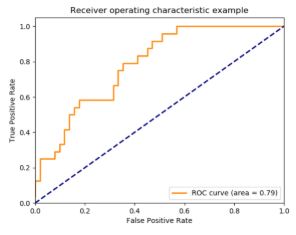
In addition to those we can look at Receiver Operating Characteristic (ROC) curves which plot the true positive rate vs the false positive rate at different threshold settings. This can be used to compare the performance of different algorithms. These are often summed up by computing the area under the ROC curve.
7.2.5.2.1. Getting basic performance metrics
Now lets get the performance metrics from our RF model we just created. We can do this by using .predict() and .predict_proba() to obtain the predictions and probabilities from our model.
# Obtain the predictions from our random forest model
predicted = model.predict(X_test)
# Predict probabilities
probs = model.predict_proba(X_test)
Next we can use roc_auc_socre() to get the ROC score, classification_report() to get the precision, recall, and f-score, and confusion_matrix() to get the confusion matrix.
# Print the ROC curve, classification report and confusion matrix
print('ROC Score:')
print(roc_auc_score(y_test, probs[:,1]))
print('\nClassification Report:')
print(classification_report(y_test, predicted))
print('\nConfusion Matrix:')
print(confusion_matrix(y_test, predicted))
Here we see we have a much higher precision (less false positives) but lower recall (more false negatives).
7.2.5.2.2. Plotting the Precision vs. Recall Curve
The Precision-Recall curve allows us to investigate the trade-off between focusing on either of the two in our model. A good model balances the two. First we will need to calculate the average precision as well as the precision and recall.
# Calculate average precision and the PR curve
average_precision = average_precision_score(y_test, predicted)
average_precision
# Obtain precision and recall
precision, recall, _ = precision_recall_curve(y_test, predicted)
print(f'Precision: {precision}\nRecall: {recall}')
Now we define a function plot_pr_curve() which will plot our precision-recall curve for us.
def plot_pr_curve(recall, precision, average_precision):
    """
    https://scikit-learn.org/stable/auto_examples/model_selection/plot_precision_recall.html
    """
    from inspect import signature
    plt.figure()
    step_kwargs = ({'step': 'post'}
                   if 'step' in signature(plt.fill_between).parameters
                   else {})

    plt.step(recall, precision, color = 'b', alpha = 0.2, where = 'post')
    plt.fill_between(recall, precision, alpha = 0.2, color = 'b', **step_kwargs)

    plt.xlabel('Recall')
    plt.ylabel('Precision')
    plt.ylim([0.0, 1.0])
    plt.xlim([0.0, 1.0])
    plt.title(f'2-class Precision-Recall curve: AP={average_precision:0.2f}')
    return plt.show()
Running this code for our data gives the following
# Plot the recall precision tradeoff
plot_pr_curve(recall, precision, average_precision)
7.2.5.3. Adjusting algorithm weights
When training a model we often want to tweak it to get the best recall-precision balance.
sklearn has simple options to tweak its models for imbalanced data relating to the class_weight parameter which can be applied to Random Forests.
class_weight = 'balanced': the model uses the values of y to automatically adjust weights inversely proportional to class frequencies in the the input data. This can also be applied to other classifiers like Logistic Regression and SVCclass_weight = 'balanced_subsample': same as balanced, except weights are calculated again at each iteration of a growing tree. This only applies to Random Forests.manual input: you can also manually adjust weights to any ratio, for example
class_weight={0:1,1:4}
7.2.5.3.1. Balanced Subsample
Lets try using the balanced_subsample option with our data. We will follow the same steps as earlier but now with class_weight = 'balanced_subsample'
# Define the model with balanced subsample
model = RandomForestClassifier(class_weight = 'balanced_subsample', random_state = 5, n_estimators = 100)

# Fit your training model to your training set
model.fit(X_train, y_train)

# Obtain the predicted values and probabilities from the model
predicted = model.predict(X_test)
probs = model.predict_proba(X_test)

# Print the ROC curve, classification report and confusion matrix
print('ROC Score:')
print(roc_auc_score(y_test, probs[:,1]))
print('\nClassification Report:')
print(classification_report(y_test, predicted))
print('\nConfusion Matrix:')
print(confusion_matrix(y_test, predicted))
Here there wasn’t much improvement. The only major change is that false positives went down by 1. This was a nice simple option to try but we can do better.
7.2.5.3.2. Hyperparamaters
Random Forest also has other options, one of which we mentioned previously. These options are called hyperparamaters as they control the learning process of the algorithm. Here is an example of specifying a few potentially important ones.
model = RandomForestClassifier(n_estimators = 10,
                               criterion = ’gini’,
                               max_depth = None,
                               min_samples_split = 2,
                               min_samples_leaf = 1,
                               max_features = ’auto’
                               n_jobs = -1
                               class_weight = None)
n_estimators: number of trees in the forest (very important)criterion: changes the way the data is split at each node, defaults to the gini coefficientmax_depth,min_samples_split,min_samples_leaf, andmax_features: some of the options determining the shape of the treesn_jobs: specifies how many jobs to do in parallel (how many processors to use). This defaults to 1, and -1 uses all processors available.class_weight: discussed previously
7.2.5.3.3. Adjusting RF manually
It is possible to get better results by assigning weights and tweaking the shape of our decision trees.
We will start by first defining a function get_model_results() which will fit a model on data and print the same preformance metrics as we have done previously.
def get_model_results(X_train: np.ndarray, y_train: np.ndarray,
                      X_test: np.ndarray, y_test: np.ndarray, model):
    """
    model: sklearn model (e.g. RandomForestClassifier)
    """
    # Fit your training model to your training set
    model.fit(X_train, y_train)

    # Obtain the predicted values and probabilities from the model
    predicted = model.predict(X_test)

    try:
        probs = model.predict_proba(X_test)
        print('ROC Score:')
        print(roc_auc_score(y_test, probs[:,1]))
    except AttributeError:
        pass

    # Print the ROC curve, classification report and confusion matrix
    print('\nClassification Report:')
    print(classification_report(y_test, predicted))
    print('\nConfusion Matrix:')
    print(confusion_matrix(y_test, predicted))
In our example we have 300 fraud to 7000 non-fraud cases, so if we set the weight ratio to 1:12 we would get 1/3 fraud to 2/3 non-fraud to train our model on each time it samples the training data.
In addition we can set the criterion to entropy, maximum tree dept to 10, minimal samples in leaf nodes to 10, and the number of trees in the model to 20 to try and get a good result. These are just used as an example, we will go over the optimization of these options later.
# Change the model options
model = RandomForestClassifier(bootstrap = True,
                               class_weight = {0:1, 1:12},
                               criterion = 'entropy',
                               # Change depth of model
                               max_depth = 10,
                               # Change the number of samples in leaf nodes
                               min_samples_leaf = 10,
                               # Change the number of trees to use
                               n_estimators = 20,
                               n_jobs = -1,
                               random_state = 5)

# Run the function get_model_results
get_model_results(X_train, y_train, X_test, y_test, model)
Here we can see the model has improved! The false negatives have gone down by 4, without compromising the false positives.
7.2.5.3.4. Parameter optimization with GridSearchCV
GridSearchCV (from sklearn.model_selection) allows us to tweak our model parameters in a more systematic way. It evaluates all combinations of parameters as defined in a parameter grid (a dictionary relating parameters to their possible values) in relation to a scoring metric (precision, recall or f1) to determine which combination is best.
We start by defining our parameter grid and define our model. Here we want to test:
1 vs 30 for number of trees
gini vs entropy for criterion
auto vs log2 for max features
4 vs 8 vs 10 vs 12 for max tree depth
# Define the parameter sets to test
param_grid = {'n_estimators': [1, 30],
              'criterion': ['gini', 'entropy'],
              'max_features': ['auto', 'log2'],
              'max_depth': [4, 8, 10, 12]}

# Define the model to use
model = RandomForestClassifier(random_state = 5)
Next we will call GridSearchCV() using our model and parameter grid to create a new model taking into account the parameter set. cv = 5 specifies our cross-validation splitting strategy as being a 5-fold cross validation. scoring = 'recall' tells the function to optimize for recall. njobs = -1 will allow GridSearchCV to use all of our processor cores to speed up the computation.
# Combine the parameter sets with the defined model
CV_model = GridSearchCV(estimator = model, param_grid = param_grid, cv = 5, scoring = 'recall', n_jobs = -1)
Finally we fit the model the same as done previously. We can use .best_params_ to get the best parameter from our fit.
# Fit the model to our training data and obtain best parameters
CV_model.fit(X_train, y_train)
CV_model.best_params_
So it appears that from our options the best criterion is 'gini', the max depth should be 8, the max features should be 'log2' and the number of trees should be 30. Now lets apply this information by adjusting the parameter as we have done before and generating a report.
# Input the optimal parameters in the model
model = RandomForestClassifier(class_weight = {0:1,1:12},
                               criterion = 'gini',
                               max_depth = 8,
                               max_features = 'log2',
                               min_samples_leaf = 10,
                               n_estimators = 30,
                               n_jobs = -1,
                               random_state = 5)

# Get results from your model
get_model_results(X_train, y_train, X_test, y_test, model)
When compared to the balanced subsample results false negatives went down by 3, however false positives also went up by three. To determine which model is best decisions should be made based on how important it is to catch fraud vs how many false positives can be dealt with.
7.2.5.4. Ensemble Methods
Ensemble methods create multiple machine learning models and combine them to produce a final result which is usually more accurate than a single model alone. These methods take into account a selection of models and average them to produce a final model. This ensures predictions are robust, there is less overfitting, and improves prediction performance (particularly in the case of models with different recall and precision scores). Many Kaggle competition winners use ensemble models.
Random Forests are an example of an ensemble method, as it is an ensemble of decision trees. It uses the bootstrap aggregation or _bagging ensemble_method for creating an ensemble method. Here models are trained on random subsamples of data and the results from each model are aggregated by taking the average prediction of all the trees.
7.2.5.4.1. Stacking Ensemble Methods
One way of creating an ensemble method is by stacking. In this multiple models are trained on the entire training dataset. These models are then combined via a “voting” method where the classification probabilities from each model are compared. This is often done with models who differ from one another, unlike bagging ensembles which often use the same type of model multiple times.
Lets try to improve upon a logistic regression model by combining it with a random forest and decision tree. First we need to establish the baseline of the logistic regression model alone the same way we have done previously.
# Define the Logistic Regression model with weights
model = LogisticRegression(class_weight = {0:1, 1:15}, random_state = 5, solver = 'liblinear')

# Get the model results
get_model_results(X_train, y_train, X_test, y_test, model)
Here we see that the logistic regression had a great deal more false positives than the random forest, but also had a better recall. This means that combing them in an ensemble method would be useful. Lets start by defining the three models we will use in our ensemble:
Logistic Regression from before
Random Forest from before
Decision Tree with balanced class weights
# Define the three classifiers to use in the ensemble
clf1 = LogisticRegression(class_weight = {0:1, 1:15},
                          random_state = 5,
                          solver = 'liblinear')

clf2 = RandomForestClassifier(class_weight = {0:1, 1:12},
                              criterion = 'gini',
                              max_depth = 8,
                              max_features = 'log2',
                              min_samples_leaf = 10,
                              n_estimators = 30,
                              n_jobs = -1,
                              random_state = 5)

clf3 = DecisionTreeClassifier(random_state = 5,
                              class_weight = "balanced")
Now we can use VotingClassifier() from sklearn.ensemble to combine the three. We can specify the voting parameter to be 'hard' or 'soft'. 'hard' will use the predicted class labels and take the majority vote (i.e. 2/3 of the models said this case is fraud, therefore it is fraud). 'soft' will take the average probability of a class by combining the individual models.
# Combine the classifiers in the ensemble model
ensemble_model = VotingClassifier(estimators = [('lr', clf1), ('rf', clf2), ('dt', clf3)],
                                  voting = 'hard')

# Get the results
get_model_results(X_train, y_train, X_test, y_test, ensemble_model)
Here we can see that the number of false positives has dramatically reduced, while we are getting the smallest amount of false negatives of any algorithm we have tried so far.
7.2.5.4.1.1. Adjusting weights within the Voting Classifier
We can potentially improve performance even more by adjusting the weights given to each model in our ensemble. This allows us to change how much emphasis we place on a particular model relative to the others. This can be done by specifying a list for the weights parameter in VotingClassifier().
# Define the ensemble model
ensemble_model = VotingClassifier(estimators = [('lr', clf1), ('rf', clf2), ('gnb', clf3)],
                                  voting = 'soft', weights = [1, 4, 1],
                                  flatten_transform = True)

# Get results
get_model_results(X_train, y_train, X_test, y_test, ensemble_model)
Playing around with weights will allow us to tweak the performance of our model even further to achieve the kind of results we are looking for. In this case it decreased the false positives by 4, but increased the false positives by 1.
7.2.6. Fraud Detection using unlabled data
Oftentimes the data we get isn’t prelabled as fraudulent. In that case we need to use unsupervised learning techniques to detect fraud.
7.2.6.1. Normal vs Abnormal Behavior
To do this we must make a distinction between normal and abnormal behavior. Abnormal behavior isn’t necessarily fraudulent, but it can be used to make a determination on how likely a case is fraud. This is generally difficult since it is difficult to validate your data.
When looking for abnormal behavior there are a few things to consider:
thoroughly describe the data:
plot histograms
check for outliers
investigate correlations
Are there any known historic cases of fraud? What typifies those cases?
Investigate whether the data is homogeneous, or whether different types of clients display different behavior
Check patterns within subgroups of data: is your data homogeneous?
Verify data points are the same type:
individuals
groups
companies
governmental organizations
Do the data points differ on:
spending patterns
age
location
frequency
For credit card fraud, location can be an indication of fraud
This goes for e-commerce sites
where’s the IP address located and where is the product ordered to ship?
7.2.6.1.1. Exploring the Data
Here we will be looking at payment transaction data. Transactions are categorized by type of expense and amount spent. We also have another data file with some information on client characteristics such as age group and gender. Some transactions have been labeled as fraud which we will use to validate our results later. To understand what is normal you need a good understanding of the data and its characteristics.
Lets get our data into some DataFrames and get an idea of what they look like.
banksim_df = pd.read_csv(banksim_file)
banksim_df.drop(['Unnamed: 0'], axis = 1, inplace = True)
banksim_adj_df = pd.read_csv(banksim_adj_file)
banksim_adj_df.drop(['Unnamed: 0'], axis = 1, inplace = True)
banksim_df.shape # 7200 rows and 5 columns
banksim_df.head()
banksim_adj_df.shape
banksim_adj_df.head()
Now we will use groupby from pandas to take a mean of the data based on transaction type.
banksim_df.groupby(['category']).mean()
Here we can already see that the majority of fraud is in travel, leisure, and sports related transactions.
7.2.6.1.2. Customer Segmentation
Lets look for some obvious patterns in the data to determine if we need to segment the data into groups or if it’s fairly homogeneous. Lets look at age groups and see if there is any significant difference in behavior.
banksim_df.groupby(['age']).mean()
banksim_df.age.value_counts()
Since the largest age groups are relatively similar, we should probably not split the data into age segments before running fraud detection.
7.2.6.1.3. Using statistics to define normal behavior
Lets see how fraudulent transactions differ structurally from normal transactions by looking at the average amounts spent. We will create two new dataframes for fraud and non fraud data then plot the two as histograms.
# Create two dataframes with fraud and non-fraud data
df_fraud = banksim_df[banksim_df.fraud == 1]
df_non_fraud = banksim_df[banksim_df.fraud == 0]

# Plot histograms of the amounts in fraud and non-fraud data
plt.hist(df_fraud.amount, alpha = 0.5, label = 'fraud')
plt.hist(df_non_fraud.amount, alpha = 0.5, label = 'nonfraud')
plt.xlabel('amount')
plt.legend()
plt.show()
Since there are less fraudulent transactions lets take a look at only a histogram of them to see their distribution.
plt.hist(df_fraud.amount, alpha = 0.5, label = 'fraud')
plt.xlabel('amount')
plt.show()
Here we see that fraudulent transactions tend to be on the larger side! This will help in distinguishing fraud from non-fraud.
7.2.6.2. Clustering methods to detect fraud
The objective of any clustering model is to detect patterns in data. Specifically it is to group the data into distinct data clusters made of points similar to each other but distinct from other points.
7.2.6.2.1. Scaling the data
For any ML algorithm using distance its crucial to always scale your data, so lets do that first. We can use MinMaxScaler from sklearn.preprocessing to scale our data.
First we will create a Numpy array from our dataframe only containing the values from df as floats.
labels = banksim_adj_df.fraud

cols = ['age', 'amount', 'M', 'es_barsandrestaurants', 'es_contents',
        'es_fashion', 'es_food', 'es_health', 'es_home', 'es_hotelservices',
        'es_hyper', 'es_leisure', 'es_otherservices', 'es_sportsandtoys',
        'es_tech', 'es_transportation', 'es_travel']

# Take the float values of df for X
X = banksim_adj_df[cols].values.astype(np.float)

X.shape
Then we can define the scaler and apply it.
# Define the scaler and apply to the data
scaler = MinMaxScaler()
X_scaled = scaler.fit_transform(X)
7.2.6.2.2. K-means clustering
K-means clustering tries to minimize the sum of all distances between the data samples and their associated cluster centroids. The score of K-means clustering is the inverse of that minimization, so should be close to 0 ideally. It is a straightforward and relatively powerful method of predicting suspicious cases. With very large data however MiniBatch K-means is a more efficient way to implement K-means and is what we will be doing.
We can use MiniBatchKMeans from sklearn to do so. We will specify that there is to be 8 clusters and set the random state to 0 to have repeatable results.
# Define the model
kmeans = MiniBatchKMeans(n_clusters = 8, random_state = 0)

# Fit the model to the scaled data
kmeans.fit(X_scaled)
7.2.6.2.3. Elbow Method for determining clusters
While we picked 8 clusters in the previous example, this might not be ideal! It’s very important to get the number of clusters correct, particularly when doing fraud detection. There are a few ways to do so, but here we apply the Elbow Method to do just that. To do this we will generate an elbow curve which scores each model and plots them vs the number of clusters in them.
In this example we will be looking at 1 to 10 clusters, running MiniBatch K-means on all the clusters in this range, fit the models, and plotting them with their respective scores
# Define the range of clusters to try
clustno = range(1, 10)

# Run MiniBatch Kmeans over the number of clusters
kmeans = [MiniBatchKMeans(n_clusters = i) for i in clustno]

# Obtain the score for each model
score = [kmeans[i].fit(X_scaled).score(X_scaled) for i in range(len(kmeans))]

# Plot the models and their respective score
plt.plot(clustno, score)
plt.xlabel('Number of Clusters')
plt.ylabel('Score')
plt.title('Elbow Curve')
plt.show()
To determine which is the ideal number of clusters we look for the elbow of the curve. That is where the score begins to increase less as the number of clusters increase. In this case it is at 3 clusters.
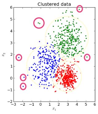
7.2.6.3. Assigning fraud vs non-fraud
The general method of assigning fraud after clustering is to take the outliers of each cluster and flag those as fraud. We do this by finding the distance of each point to their cluster’s centroid and establishing a cutoff distance beyond which a point is an outlier (i.e. 95%). These outliers are abnormal or suspicious, but aren’t necessarily fraudulent.
7.2.6.3.1. Detecting Outliers
To do this first we will split our data into training and testing sets as we have done before.
# Split the data into training and test set
X_train, X_test, y_train, y_test = train_test_split(X_scaled, labels, test_size = 0.3, random_state = 0)
Then we will define our K-means model with 3 clusters as we determined with the elbow test.
# Define K-means model
kmeans = MiniBatchKMeans(n_clusters = 3, random_state = 42).fit(X_train)
Now we need to get the cluster predictions as well as the cluster centroids.
# Obtain predictions and calculate distance from cluster centroid
X_test_clusters = kmeans.predict(X_test)
X_test_clusters_centers = kmeans.cluster_centers_
dist = [np.linalg.norm(x-y) for x, y in zip(X_test, X_test_clusters_centers[X_test_clusters])]
Finally we define the boundry between fraud and non-fraud at 95% of the distance distribution or higher.
# Create fraud predictions based on outliers on clusters
km_y_pred = np.array(dist)
km_y_pred[dist >= np.percentile(dist, 95)] = 1
km_y_pred[dist < np.percentile(dist, 95)] = 0
7.2.6.3.2. Checking model results
Lets create some preformance metrics to see how well this was at detecting fraud.
Lets define a function that can create a nice looking confusion matrix first.
def plot_confusion_matrix(cm, classes = ['Not Fraud', 'Fraud'],
                          normalize = False,
                          title = 'Fraud Confusion matrix',
                          cmap = plt.cm.Blues):
    """
    This function prints and plots the confusion matrix.
    Normalization can be applied by setting `normalize=True`.
    From:
        http://scikit-learn.org/stable/auto_examples/model_selection/plot_confusion_matrix.html#sphx-glr-auto-
        examples-model-selection-plot-confusion-matrix-py
    """
    if normalize:
        cm = cm.astype('float') / cm.sum(axis = 1)[:, np.newaxis]
        print("Normalized confusion matrix")
    else:
        print('Confusion matrix, without normalization')

    # print(cm)

    plt.imshow(cm, interpolation = 'nearest', cmap = cmap)
    plt.title(title)
    plt.colorbar()
    tick_marks = np.arange(len(classes))
    plt.xticks(tick_marks, classes, rotation = 45)
    plt.yticks(tick_marks, classes)

    fmt = '.2f' if normalize else 'd'
    thresh = cm.max() / 2.
    for i, j in product(range(cm.shape[0]), range(cm.shape[1])):
        plt.text(j, i, format(cm[i, j], fmt),
                 horizontalalignment = "center",
                 color = "white" if cm[i, j] > thresh else "black")

    plt.tight_layout()
    plt.ylabel('True label')
    plt.xlabel('Predicted label')
    plt.show()
Now lets get the ROC score and confusion matrix
print('ROC Score:')
print(roc_auc_score(y_test, km_y_pred))
print()

# Create a confusion matrix
km_cm = confusion_matrix(y_test, km_y_pred)

# Plot the confusion matrix in a figure to visualize results
plot_confusion_matrix(km_cm)
This wasn’t nearly as good as our models created with labled data, however it does work for detecting fraud!
7.2.6.4. Other methods: DBSCAN
K-means works well with data clustered into normal, round shapes but has it’s downsides. It can’t handle any data clusters not in that shape. It can also end up identifying multiple outliers as their own smaller cluster. There are many other clustering methods out there.
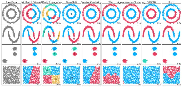
One that we will look at today is DBSCAN. DBSCAN stands for Density-Based Spatial Clustering of Applications with Noise. It does not require the number of clusters to be predefined. Instead it finds core samples of high density and expands clusters from them. This means it works well with data containing clusters of similar density. It can be used to ID fraud as very small clusters. It does require you to assign the maximum allowed distance between points in a cluster and the minimum points which constitute a cluster. It has the best performance on weirdly shaped data, however it is computationally heavier than MiniBatch K-means.
7.2.6.4.1. Implementing DBSCAN
DBSCAN is available from sklearn.cluster. We will need to set the max distance between samples (0.9) and minimum observations (10) to fit our data.
# Initialize and fit the DBscan model
db = DBSCAN(eps = 0.9, min_samples = 10, n_jobs = -1).fit(X_scaled)
Now lets see how many clusters we have and the preformance metrics.
# Obtain the predicted labels and calculate number of clusters
pred_labels = db.labels_
n_clusters = len(set(pred_labels)) - (1 if -1 in labels else 0)

# Print performance metrics for DBscan
print(f'Estimated number of clusters: {n_clusters}')
print(f'Homogeneity: {homogeneity_score(labels, pred_labels):0.3f}')
print(f'Silhouette Coefficient: {silhouette_score(X_scaled, pred_labels):0.3f}')
7.2.6.4.2. Assessing smallest clusters
We now need to filter out the smallest clusters from the 23 we identified. We will start by counting the samples in each cluster by running a bincount on the cluster numbers under pred_labels.
# Count observations in each cluster number
counts = np.bincount(pred_labels[pred_labels >= 0])

# Print the result
print(counts)
We will then sort counts and take the three smallest clusters.
# Sort the sample counts of the clusters and take the top 3 smallest clusters
smallest_clusters = np.argsort(counts)[:3]

# Print the results
print(f'The smallest clusters are clusters: {smallest_clusters}')
Within counts, we will select only these smallest clusters and print the number of samples in each.
# Print the counts of the smallest clusters only
print(f'Their counts are: {counts[smallest_clusters]}')
7.2.6.4.3. Verifying our Results
While in reality you usually don’t have labels to do this, we can verify our results to see how well DBSCAN did.
First we will create a dataframe combining the cluster numbers and their actual labels.
# Create a dataframe of the predicted cluster numbers and fraud labels
df = pd.DataFrame({'clusternr':pred_labels,'fraud':labels})
Next we will create a condition that flags fraud for the three smallest clusters: 21, 17, and 9.
# Create a condition flagging fraud for the smallest clusters
df['predicted_fraud'] = np.where((df['clusternr'].isin([21, 17, 9])), 1 , 0)
Finally we run a crosstab on our results
# Run a crosstab on the results
print(pd.crosstab(df['fraud'], df['predicted_fraud'],
                  rownames = ['Actual Fraud'],
                  colnames = ['Flagged Fraud']))
For our flagged cases roughly 2/3 are actually fraud! Because we only took the three smallest clusters we flag less cases of fraud, causing more false negatives. We could increase this number, however this will risk increasing the number of false positives in turn.
7.2.7. Cleaning up
Now that we are done using our data files we are going to get rid of them. I hope this was informative!
# if os.path.exists("data/chapter_1"):
#     shutil.rmtree("data/chapter_1")

# if os.path.exists("data/chapter_2"):
#     shutil.rmtree("data/chapter_2")

# if os.path.exists("data/chapter_3"):
#     shutil.rmtree("data/chapter_3")

# if os.path.exists("data/chapter_4"):
#     shutil.rmtree("data/chapter_4")