7.9. Neural Networks in Python
7.9.1. What is a Neural Network?
In these notes we will be implementing a predictive Neural Network in Python. Artificial Neural Networks are a specific type of machine learning model loosely based on the Biological Neural Networks that our own brains run on. Neural Networks have seen extremely broad applications including but not limited to pattern recognition, medical diagnostics, geosciences, cybersecurity, and quantum chemistry.
At their core, Neural Networks consist of the following:
An input layer, \(x\)
An arbitrary amount of hidden layers comprised of nodes which process data from previous layers
An output layer, \(\hat{y}\)
A set of weights and biases connecting the nodes in each layer, \(W\) and \(b\)
An activation function for each hidden layer, \(\sigma\), which takes the layers’ input and outputs a value between 0 and 1 (or -1 and 1).
These layers act to progressively extract higher level features from raw input in a process known as Deep Learning (so long as there is more than two hidden layers). A simplified diagram of a Neural Network is shown below. You can see the input layer on the left which is inputted into the hidden layer in the middle, which outputs to the output layer and classifies the image.

There can be any number of hidden layers and nodes in each layer, and multiple different activation functions (linear, sigmoid, etc.) can be used. Part of the challenge of successfully implementing a Neural Network is determining these things.
7.9.2. Training a Neural Network
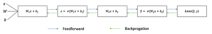
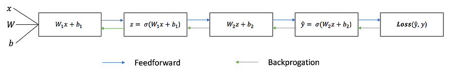
Another key part of a neural network is its ability to self train. Commonly this is done in two steps that are repeated until the desired performance is achieved.
Calculating the predicted output \(\hat{y}\), called feedforward
Updating the weights \(W\) and biases \(b\), called backpropogation
This allows Neural Networks to learn so long as they have already classified data to be trained on. An diagram of what this looks like with a one layer Neural Network is shown below. Here we can see the input \(x\), as well as the weights \(W\) and biases \(b\) used at the start which are used to feedforward and get the \(\hat{y}\). Then the weights and biases are updated based on the derivative of the loss function.
Generally training a Neural Network will occur over Epochs split into Batches. An Epoch is one pass through all rows of the training dataset. A Batch is one (or more) samples considered by the model within an epoch before updating weights (backpropogation).
7.9.3. Keras: A Python Module for Neural Networks
Keras is a versatile module for python to implement neural networks.
7.9.3.1. Install Keras:
Please install package below beforehand and dependencies.
#!pip3 install keras
#!pip3 install tensorflow
#!pip3 install uszipcode
7.9.3.2. Load Data
import numpy as np
import pandas as pd
from sklearn import linear_model
import datetime
import seaborn as sns
from uszipcode import SearchEngine
from sklearn.preprocessing import OneHotEncoder, OrdinalEncoder
from sklearn.compose import ColumnTransformer
from sklearn.metrics import confusion_matrix, ConfusionMatrixDisplay

from keras.models import Sequential
from keras.layers import Dense
from keras.utils.vis_utils import plot_model
train = pd.read_csv("kaggle/input/train_2021.csv")
This dataset has a number of non-numeric variables that need to be properly processed first. This is borrowed from a previous version of my group’s Travelers competition work.
train.marital_status.fillna(1.0, inplace = True)    # fill the five values with majority
train.witness_present_ind.fillna(0.0, inplace = True)  # fill with majority as well as witness not present when na
train.age_of_vehicle.fillna(5, inplace = True)

input_mod1 = linear_model.LinearRegression()
input_mod1.fit(train.loc[train.claim_est_payout.isna() == False, ['vehicle_price', 'age_of_vehicle']],
               train.claim_est_payout[train.claim_est_payout.isna() == False])

# predicted values for NA's
input_output = pd.Series(input_mod1.predict(train.loc[train.claim_est_payout.isna() == True,
                                                      ['vehicle_price', 'age_of_vehicle']]),
                         index = train.index[train.claim_est_payout.isna()==True])

train.claim_est_payout.fillna(input_output, inplace = True)

train['claim_date_d'] = pd.Series([datetime.datetime.strptime(d, '%m/%d/%Y').strftime('%d')
                                   for d in train.claim_date], index = train.index)
train['claim_date_m'] = pd.Series([datetime.datetime.strptime(d, '%m/%d/%Y').strftime('%m')
                                   for d in train.claim_date], index = train.index)

# Capping 'age_of_driver' at 80
train['age_of_driver'] = train['age_of_driver'].clip(upper = 80)

# fitting regression of claim_est_payout using vehicle_price and `age_of_vehicle`

input_mod2 = linear_model.LinearRegression()
input_mod2.fit(train.loc[train.annual_income != -1, ['age_of_driver']],
               train.annual_income[train.annual_income != -1])

# predicted values for -1's
input_output2 = pd.Series(input_mod2.predict(train.loc[train.annual_income == -1,
                                                      ['age_of_driver']]),
                         index = train.index[train.annual_income == -1])

# replacing -1 values with predicted values
train.annual_income.replace(to_replace = ([-1] * len(input_output2)),
                            value = input_output2, inplace = True)

engine = SearchEngine()

def zip_lookup(row):
    if row.zip_code == 0:
        return pd.DataFrame(data = {
                "state" : [np.nan],
                "lat" : [np.nan],
                "lng" : [np.nan]
               })
    else:
        info = engine.by_zipcode(str(row.zip_code))
        # changing to pandas dataframe
        return pd.DataFrame(data = {
                "state" : [info.state],
                "lat" : [info.lat],
                "lng" : [info.lng]
               })

train["state"] = train.apply(lambda row: zip_lookup(row).at[0, 'state'], axis = 1)
train["latitude"] = train.apply(lambda row: zip_lookup(row).at[0, 'lat'], axis = 1)
train["longitude"] = train.apply(lambda row: zip_lookup(row).at[0, 'lng'], axis = 1)

train["state"] = train.state.fillna(method = "bfill")
train["latitude"] = train.latitude.fillna(method = "bfill")
train["longitude"] = train.longitude.fillna(method = "bfill")

train_encoded = pd.DataFrame()

# modify all numerical to binned variables
train_encoded['claim_number'] = train['claim_number'].astype('category')
train_encoded['dr_age_bins'] = pd.cut(train.age_of_driver,
                                      bins = train.age_of_driver.quantile([0, .05, .25, .75, .95, 1]),
                                      include_lowest = True)
train_encoded['dr_safty_bins'] = pd.cut(train.safty_rating,
                                        bins = train.safty_rating.quantile([0, .1, .3, .8, .95, 1]),
                                        include_lowest = True)
train_encoded['dr_annual_income'] = pd.cut(train.annual_income,
                                           bins = train.annual_income.quantile([0, .1, .3, .8, .95, 1]),
                                           include_lowest = True)
train_encoded['zip_code_1'] = round(train.zip_code/10000, 0).astype('category')    # satisfy the same state
train_encoded['past_num_of_claims'] = pd.cut(train.past_num_of_claims,
                                             bins = train.past_num_of_claims.quantile([0, 0.8, 0.9, 1]),
                                             include_lowest = True) # ordinal
train_encoded['liab_prct'] = pd.cut(train.liab_prct,
                                    bins = train.liab_prct.quantile([0, 0.25, 0.75, 1]),
                                    include_lowest = True)
train_encoded['claim_est_payout'] = pd.cut(train.claim_est_payout,
                                           bins = train.claim_est_payout.quantile([0, 0.05, .25, .75, .95, 1]),
                                           include_lowest = True)
train_encoded['age_of_vehicle'] = pd.cut(train.age_of_vehicle,
                                         bins = train.age_of_vehicle.quantile([0, .25, .75, .9, 1]),
                                         include_lowest = True)
train_encoded['vehicle_price'] = pd.cut(train.vehicle_price,
                                        bins = train.vehicle_price.quantile([0, .1, .25, .75, .9, 1]),
                                        include_lowest = True)
train_encoded['vehicle_weight'] = pd.cut(train.vehicle_weight,
                                         bins = train.vehicle_weight.quantile([0, .1, .25, .75, .9, 1]),
                                         include_lowest = True)

# not binned numeric
train_encoded['latitude'] = train['latitude']
train_encoded['longitude'] = train['longitude']


# derived variables as categorical
# train_encoded['claim_date_d'] = train['claim_date_d'].astype('category')
# train_encoded['claim_date_m'] = train['claim_date_m'].astype('category')

# already categorical variables
train_encoded['gender'] = train['gender']
train_encoded['marital_status'] = train['marital_status'].astype('category')
train_encoded['high_education_ind'] = train['high_education_ind'].astype('category')
train_encoded['address_change_ind'] = train['address_change_ind'].astype('category')
train_encoded['living_status'] = train['living_status']
train_encoded['claim_day_of_week'] = train['claim_day_of_week']
train_encoded['witness_present_ind'] = train['witness_present_ind'].astype('category')
train_encoded['channel'] = train['channel']
train_encoded['policy_report_filed_ind'] = train['policy_report_filed_ind'].astype('category')
train_encoded['vehicle_category'] = train['vehicle_category']
train_encoded['vehicle_color'] = train['vehicle_color']
train_encoded['state'] = train['state'].astype('category')
train_encoded['fraud'] = train['fraud'].astype('category')

list_ordinal = ['dr_safty_bins', 'dr_annual_income', 'past_num_of_claims','liab_prct',
                'claim_est_payout', 'age_of_vehicle', 'vehicle_price', 'vehicle_weight']
list_other = ['dr_age_bins', 'zip_code_1', 'gender', 'marital_status', 'high_education_ind',
              'address_change_ind', 'living_status', 'claim_day_of_week',
              'witness_present_ind', 'channel', 'policy_report_filed_ind', 'vehicle_category',
              'vehicle_color', 'state']

encoding = [('ord', OrdinalEncoder(), list_ordinal), ('cat', OneHotEncoder(), list_other)]
# encoding = [('ord', OneHotEncoder(), list_ordinal), ('cat', OneHotEncoder(), list_other)]
col_transform = ColumnTransformer(transformers = encoding)

X = train_encoded.iloc[:, 1:-1]
y = train_encoded.iloc[:,  -1]

X_1 = col_transform.fit_transform(X)

from sklearn.model_selection import train_test_split
X_in1, X_hold1, y_in, y_hold = train_test_split(X_1, y, test_size=0.3, random_state=341)
X_in1.shape
7.9.3.3. Defining the Keras Model
As discussed previously, Neural Networks are defined as a sequence of layers. In this example we will be creating a Sequential model where we will add one layer at a time until we are satisfied with the network structure. This is done by defining a new model using the Sequential() class from Keras.
Knowing how many layers to add and their structure is a challenging problem, and is often best solved through trial and error. Though generally a Neural Network should be large enough to reflect the structure of the problem. In this example we will be using a fully connected structure (Each layers’ nodes connect to every node in the layers behind and ahead of them) with 5 layers.
model = Sequential()
Now we will add our layers. Our input layer will be defined in the same command as our first hidden layer. This input layer will have a number of input features (nodes) equal to the number of input variables we have, in this case 57. We do this with the input_dim argument when adding our first layer.
We will add a layer to our model using the .add() method. For a fully connected structure we need to use the Dense() class. The first argument for Dense() specifies the number of nodes in that layer. The activation argument tells the network which activation function to use in that layer.
For activation functions in the hidden layers we will be using the rectified linear unit activation function (relu) which is fairly common.
With that out of the way lets define our first layers.
model.add(Dense(86, input_dim = 57, activation = "relu"))
model.add(Dense(57, activation = "relu"))
model.add(Dense(28, activation = "relu"))
model.add(Dense(14, activation = "relu"))
Now all that’s left is to define our output layer. Since this is a classification problem our output layer will have only 1 node, as we only are looking for a single output. We will also use a sigmoid activation function instead.
model.add(Dense(1, activation = "sigmoid"))
7.9.3.4. Compiling the Keras Model
Now the model must be compiled using the .compile() method. When doing so we must also define a few things relating to the training of the network:
The loss function: This is used to specify how we will evaluate our network during training, defined with the
lossargumentThe optimizer: How our network will optimize itself, defined with the
optimizerargumentThe metrics: Any other metrics we want the model to output, defined with the
metricsargument as a list
In this example we will use "binary_crossentropy" as our loss function since this is a classification problem. For an optimizer we will use the stochastic gradient descent algorithm "adam". Finally as a metric we will add "BinaryAccuracy".
model.compile(loss = "binary_crossentropy", optimizer = "adam", metrics = ["BinaryAccuracy"])
7.9.3.5. Fitting the Keras Model
To fit our network model, we will use the .fit() method. Doing so we must specify the number of epochs we will iterate through, as well as the size of each batch within each epoch. These are defined using the epochs and batch_size arguments within this method.
For this example lets use 100 epochs with a batch size of 100.
model.fit(X_in1, y_in, epochs = 100, batch_size = 100)
If you find the reporting on each individual epoch too much, you can always add in verbose = 0 as an argument to prevent it from doing so.
7.9.3.6. Evaluating the Keras Model
Now that we have trained our Neural Network, we can test it on our test data. We will do this using the .evaluate() method. Because of how we compiled our model, this will output both the results of the loss function and the accuracy.
loss, accuracy = model.evaluate(X_hold1, y_hold)
7.9.3.7. Making Predictions using the Keras Model
We can also use the model to get predictions using the .predict() method. This will output a numpy array of the probabilities for each row, which we could either round (as we do here) or pass through some threshold to get our results. Here we do so on our split test data and create a confusion table to see how well we did.
y_pred = model.predict(X_hold1)
y_pred_r =[round(x[0]) for x in y_pred]

disp = ConfusionMatrixDisplay(confusion_matrix(y_hold, y_pred_r))
disp.plot()
This isn’t necessarily the best result, there is likely some issues with how the input data was handled and the structure of the network.
7.9.3.8. F1-Score
from sklearn.metrics import f1_score

round(f1_score(y_hold, y_pred_r), 6)
Citations:
Towards Datascience. (2018, May 17). Neural Networks [Gif]. How to Build Your Own Neural Network from Scratch in Python. https://miro.medium.com/max/2400/1*36MELEhgZsPFuzlZvObnxA.gif
Towards Datascience. (2018b, May 17). Sequential Graph [Graph]. How to Build Your Own Neural Network from Scratch in Python. https://miro.medium.com/max/933/1*CEtt0h8Rss_qPu7CyqMTdQ.png