7.10. Neural Network and Deep Learning
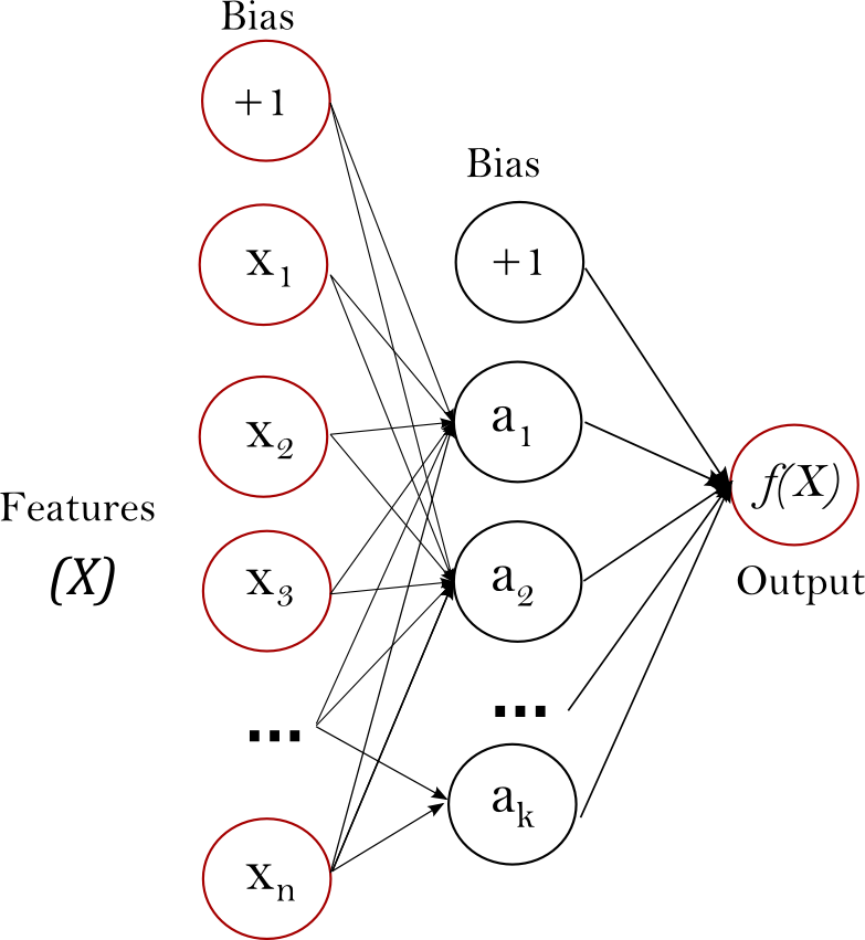
Neural Networks are described as a mathematical function that maps a given input to a desired output
Neural Networks consist of the following components
An input layer, x
An arbitrary amount of hidden layers
An output layer, ŷ
A set of weights and biases between each layer, W and b
A choice of activation function for each hidden layer, σ. In this tutorial, we’ll use a Sigmoid activation function.
 (Image by James Loy)
Each iteration of the training process consists of the following steps:
Calculating the predicted output ŷ, known as feedforward
Updating the weights and biases, known as backpropagation
Our goal in training is to find the best set of weights and biases that minimizes the loss function.
7.10.1. Application
scikit-learn is one library that has neural network. In addition,deep Learning libraries such as TensorFlow and Keras also could build neural networks.
7.10.1.1. Multi-layer Perceptron
 (Image by Scikit-learn)
7.10.1.1.1. Mathematical Formulation
7.10.1.1.2. Algorithms
7.10.1.1.3. Choices of Loss Function
class sklearn.neural_network.MLPClassifier(hidden_layer_sizes=(100), activation=’relu’, *, solver=’adam’, alpha=0.0001, batch_size=’auto’, learning_rate=’constant’, learning_rate_init=0.001, power_t=0.5, max_iter=200, shuffle=True, random_state=None, tol=0.0001, verbose=False, warm_start=False, momentum=0.9, nesterovs_momentum=True, early_stopping=False, validation_fraction=0.1, beta_1=0.9, beta_2=0.999, epsilon=1e-08, n_iter_no_change=10, max_fun=15000) details
from sklearn.datasets import load_iris
from sklearn.neural_network import MLPClassifier
from sklearn.model_selection import train_test_split
from sklearn.preprocessing import StandardScaler
import pandas as pd
from sklearn.metrics import plot_confusion_matrix
import matplotlib.pyplot as plt
from sklearn.metrics import classification_report
iris_data = load_iris()
X = pd.DataFrame(iris_data.data, columns=iris_data.feature_names)
y = iris_data.target
X_train, X_test, y_train, y_test = train_test_split(X,y,random_state=1, test_size=0.2)
sc_X = StandardScaler()
X_trainscaled=sc_X.fit_transform(X_train)
X_testscaled=sc_X.transform(X_test)
# As MLP running time is too long, the code is masked.
# clf = MLPClassifier(hidden_layer_sizes=(256,128,64,32),activation="relu",random_state=1).fit(X_trainscaled, y_train)
# y_pred=clf.predict(X_testscaled)
# print(clf.score(X_testscaled, y_test))
# print(classification_report(y_test,y_pred))
7.10.1.2. Deep learning
There are many deep learning libraries out there, but the most popular ones are TensorFlow, Keras, and PyTorch.
7.10.1.2.1. Relationship between ANN and DNN
A deep neural network (DNN) is an artificial neural network (ANN) with multiple layers between the input and output layers.
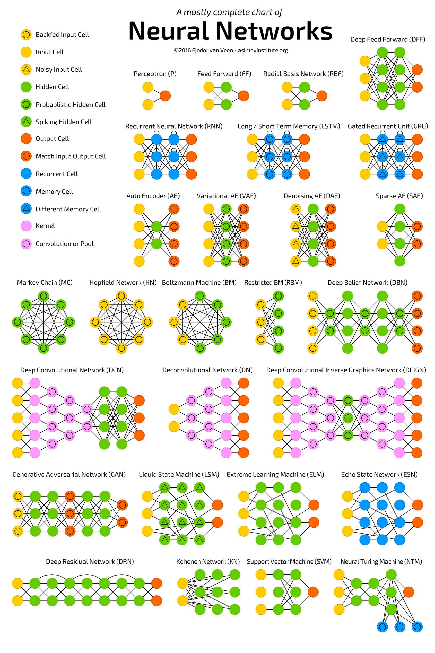
Deep Neural Networks (DNNs)
Deep Neural Networks (DNNs) are typically Feed Forward Networks (FFNNs) in which data flows from the input layer to the output layer without going backward and the links between the layers are one way which is in the forward direction and they never touch a node again
A multilayer perceptron (MLP) is a class of feedforward artificial neural network (ANN)
Recurrent Neural Network (RNN)
A Recurrent Neural Network (RNN) addresses this issue which is a FFNN with a time twist.
LSTMs are a special kind of RNN, capable of learning long-term dependencies which make RNN smart at remembering things that have happened in the past and finding patterns across time to make its next guesses make sense.
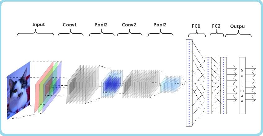
Convolutional Neural Network (CNN, or ConvNet) is a class of deep neural networks which is most commonly applied to analyzing visual imagery.
 (Image By Zhihu)
Details
Cov2d:This layer creates a convolution kernel that is convolved with the layer input to produce a tensor of outputs.
LeakyReLU: Leaky version of a Rectified Linear Unit
MaxPooling2D: Downsamples the input along its spatial dimensions (height and width)
by taking the maximum value over an input window (of size defined by pool_size) for
each channel of the input. The window is shifted by strides along each dimension.
Flatten: Flattens the input. Does not affect the batch size.
Dense: implements the operation: output = activation(dot(input, kernel) + bias)
where activation is the element-wise activation function passed as the activation argument,
kernel is a weights matrix created by the layer, and bias is a bias vector created
by the layer (only applicable if use_bias is True). These are all attributes of Dense.
# !pip install keras
from keras.datasets import fashion_mnist
(train_X,train_Y), (test_X,test_Y) = fashion_mnist.load_data()
import numpy as np
import pandas as pd
from tensorflow.keras.utils import to_categorical
import matplotlib.pyplot as plt
%matplotlib inline
from tensorflow import keras
print('Training data shape : ', train_X.shape, train_Y.shape)

print('Testing data shape : ', test_X.shape, test_Y.shape)
# Find the unique numbers from the train labels
classes = np.unique(train_Y)
nClasses = len(classes)
print('Total number of outputs : ', nClasses)
print('Output classes : ', classes)
plt.figure(figsize=[5,5])

# Display the first image in training data
plt.subplot(121)
plt.imshow(train_X[0,:,:], cmap='gray')
plt.title("Ground Truth : {}".format(train_Y[0]))

# Display the first image in testing data
plt.subplot(122)
plt.imshow(test_X[0,:,:], cmap='gray')
plt.title("Ground Truth : {}".format(test_Y[0]))
train_X = train_X.reshape(-1, 28,28, 1) # to make a transform from 784 vectors to a 28*28*1 matrix
test_X = test_X.reshape(-1, 28,28, 1)
train_X.shape, test_X.shape
train_X = train_X.astype('float32') # scaling
test_X = test_X.astype('float32')
train_X = train_X / 255.
test_X = test_X / 255.
# Change the labels from categorical to one-hot encoding
train_Y_one_hot = to_categorical(train_Y)
test_Y_one_hot = to_categorical(test_Y)

# Display the change for category label using one-hot encoding
print('Original label:', train_Y[0])
print('After conversion to one-hot:', train_Y_one_hot[0])
from sklearn.model_selection import train_test_split
train_X,valid_X,train_label,valid_label = train_test_split(train_X, train_Y_one_hot, test_size=0.2, random_state=13)
train_X.shape,valid_X.shape,train_label.shape,valid_label.shape
import keras
from keras.models import Sequential,Input,Model
from keras.layers import Dense, Dropout, Flatten
from keras.layers import Conv2D, MaxPooling2D
from keras.layers import BatchNormalization
from keras.layers.advanced_activations import LeakyReLU
import tensorflow as tf
batch_size = 64
epochs = 20
num_classes = 10
fashion_model = Sequential()
fashion_model.add(Conv2D(32, kernel_size=(3, 3),activation='linear',input_shape=(28,28,1),padding='same'))
fashion_model.add(LeakyReLU(alpha=0.1))
fashion_model.add(MaxPooling2D((2, 2),padding='same'))
fashion_model.add(Conv2D(64, (3, 3), activation='linear',padding='same'))
fashion_model.add(LeakyReLU(alpha=0.1))
fashion_model.add(MaxPooling2D(pool_size=(2, 2),padding='same'))
fashion_model.add(Conv2D(128, (3, 3), activation='linear',padding='same'))
fashion_model.add(LeakyReLU(alpha=0.1))
fashion_model.add(MaxPooling2D(pool_size=(2, 2),padding='same'))
fashion_model.add(Flatten())
fashion_model.add(Dense(128, activation='linear'))
fashion_model.add(LeakyReLU(alpha=0.1))
fashion_model.add(Dense(num_classes, activation='softmax'))
fashion_model.compile(loss=keras.losses.categorical_crossentropy, optimizer=tf.keras.optimizers.Adam(),metrics=['accuracy'])
fashion_model.summary()
# As CNN running time is too long, the code is masked.
# fashion_train = fashion_model.fit(train_X, train_label, batch_size=batch_size,epochs=epochs,verbose=1,validation_data=(valid_X, valid_label))
# As CNN running time is too long, the code is masked.
# test_eval = fashion_model.evaluate(test_X, test_Y_one_hot, verbose=0)
# print('Test loss:', test_eval[0])
# print('Test accuracy:', test_eval[1])
# As CNN running time is too long, the code is masked.
# accuracy = fashion_train.history['accuracy']
# val_accuracy = fashion_train.history['val_accuracy']
# loss = fashion_train.history['loss']
# val_loss = fashion_train.history['val_loss']
# epochs = range(len(accuracy))
# plt.plot(epochs, accuracy, 'bo', label='Training accuracy')
# plt.plot(epochs, val_accuracy, 'b', label='Validation accuracy')
# plt.title('Training and validation accuracy')
# plt.legend()
# plt.figure()
# plt.plot(epochs, loss, 'bo', label='Training loss')
# plt.plot(epochs, val_loss, 'b', label='Validation loss')
# plt.title('Training and validation loss')
# plt.legend()
# plt.show()
#predicted_classes = fashion_model.predict(test_X)
#predicted_classes = np.argmax(np.round(predicted_classes),axis=1)
#predicted_classes.shape, test_Y.shape
#correct = np.where(predicted_classes==test_Y)[0]
#print ("Found %d correct labels" % len(correct))
#for i, correct in enumerate(correct[:9]):
#    plt.subplot(3,3,i+1)
#    plt.imshow(test_X[correct].reshape(28,28), cmap='gray', interpolation='none')
#    plt.title("Predicted {}, Class {}".format(predicted_classes[correct], test_Y[correct]))
#    plt.tight_layout()
7.10.1.2.2. Unsupervised Pre-trained Neural Networks
7.10.1.2.2.1. Deep Generative Models
Boltzmann Machines/Deep Belief Neural Networks/Generative Adversarial Networks
7.10.1.2.2.2. Auto-encoder
7.10.1.2.3. Extension
Andrew Yan-Tak Ng
popular courses on Coursera are Ng’s: Machine Learning (#1), AI for Everyone, (#5), Neural Networks and Deep Learning (#6)