STAT 5361: Statistical Computing, Fall 2019
2020-12-04
Chapter 1 Prerequisites
We assume that students can use R/Rstudio comfortably. If you are new to R, an extra amount of hard work should be devoted to make it up. In addition to the official documentations from the R-project, the presentations at a local SIAM workshop in Spring 2018 given by Wenjie Wang, a PhD student in Statistics at the time, can be enlighting: - https://github.com/wenjie2wang/2018-01-19-siam - https://github.com/wenjie2wang/2018-04-06-siam
If you have used R, but never paid attention to R programming styles, a style clinic would be a necessary step. A good place to start Hadley Wickham’s tidyverse style guide at http://style.tidyverse.org/. From my experience, the two most commonly overlooked styles for beginners are spacing and indentation. Appropriate spacing and indentation would immediately make crowdly piled code much more eye-friendly. Such styles can be automatically enforced by R packages such as formatr or lintr. Two important styles that cannot be automatically corrected are naming and documentation. As in any programming languate, naming of R objects (variables, functions, files, etc.) shoud be informative, concise, and consistent with certain naming convention. Documentation needs to be sufficient, concise, and kept close to the code; tools like R package roxygen2 can be very helpful.
For intermediate R users who want a skill lift, The Advanced R Programming book (Wickham 2019) by Hadley Wickham is available at https://adv-r.hadley.nz/. The source that generated the book is kindly made available at GitHub: https://github.com/hadley/adv-r. It is a great learning experience to complile the book from the source, during which you may pick up many necessary skills. To make R work efficiently, a lot of skills are needed. Even an experienced user would find unified resources of efficient R programming (Gillespie and Lovelace 2016) useful: https://csgillespie.github.io/efficientR/.
The homework, exam, and project will be completed by R Markdown. Following the step by step the instructions in Yihui Xie’s online book on bookdown (Xie 2016).at https://bookdown.org/yihui/bookdown/, you will be amazed how quickly you can learn to produce cool-looking documents and even book manuscripts. If you are a keener, you may as well follow Yihui’s blogdown (Xie, Thomas, and Hill 2017), see the online book https://bookdown.org/yihui/blogdown/, to build your own website using R Markdown.
All your source code will be version controlled by git and archived on GitHub. RStudio has made using git quite straightforward. The online tutorial by Jenny Bryan, Happy Git and GitHub for the useR at https://happygitwithr.com/, is a very useful tool to get started
1.2 Computer Arithmetics
Burns (2012) summarizes many traps beginners may fall into. The first one is the floating number trap. Are you surprised by what you see in the following?
## [1] FALSE## [1] FALSE FALSE FALSE FALSE FALSE FALSE FALSE FALSE FALSE FALSE FALSE## [1] 0.0 0.1 0.2 0.3 0.4 0.5 0.6 0.7 0.8 0.9 1.0## [1] 0.3 0.3 0.3## [1] 0.3 0.3 0.3 0.3 0.3## [1] 0.10000000000000000555## [1] 0.099999999999999991673How does a computer represent a number? Computers use switches, which has only two states, on and off, to represent numbers. That is, it uses the binary number system. With a finite (though large) number switches on a computer, not all real numbers are representable. Binary numbers are made of bits, each of which represent a switch. A byte is 8 bits, which represents one character.
1.2.1 Integers
An integer on many computers has length 4-byte or 32-bit. It is represented by the coefficients \(x_i\) in \[ \sum_{i=1}^{32} x_i 2^{i-1} - 2^{31}, \] where \(x_i\) is either 0 or 1.
## [1] 2147483647## Warning in imax + 1L: NAs produced by integer overflow## [1] NA## [1] 30.999999999328192501## Warning in b * 2L: NAs produced by integer overflow## [1] 2147483647## [1] 1000000000## Warning in 1000L * 1000L * 1000L * 1000L: NAs produced by integer overflow## [1] NA## [1] 1e+121.2.2 Floating Point
A floating point number is represented by \[ (-1)^{x_0}\left(1 + \sum_{i=1}^t x_i 2^{-i}\right) 2^{k} \] for \(x_i \in \{0, 1\}\), where \(k\) is an integer called the exponent, \(x_0\) is the sign bit. The fractional part \(\sum_{i=1}^t x_i 2^{-i}\) is the significand. By convention (for unique representation), the exponent is chosen so that the fist digit of the significand is 1, unless it would result in the exponent being out of range.
A standard double precision representation uses 8 bytes or 64 bits: a sign bit, an 11 bit exponent, and \(t = 52\) bits for the significand. With 11 bits there are \(2^{11} = 2048\) possible values for the exponent, which are usually shifted so that the allowed values range from \(-1022\) to 1023, again with one special sign value.
The IEEE standard for floating point arithmetic calls for basic arithmetic operations to be performed to higher precision, and then rounded to the nearest representable floating point number.
Arithmetic underflow occurs where the result of a calculation is a smaller number than what the computer can actually represent. Arithmetic overflow occurs when a calculation produces a result that is greater in magnitude than what the computer can represent. Here is a demonstration (Gray 2001).
## [1] 2.2204460492503130808e-16## [1] 2.2204460492503130808e-16## [1] FALSE## [1] TRUE## [1] 0.99999999999999988898## and the largest possible exponent--note that calculating 2^1024
## directly overflows
u * 2 * 2 ^ 1023## [1] 1.7976931348623157081e+308## [1] Inf## [1] 4.9406564584124654418e-324## [1] 01.2.3 Error Analysis
More generally, a floating point number with base \(\beta\) can be represented as \[ (-1)^{x_0}\left(\sum_{i=1}^t x_i \beta^{-i}\right) \beta^{k}, \] where \(x_0 \in \{0, 1\}\), \(x_i \in \{0, 1, \ldots, \beta - 1\}\), \(i = 1, \ldots, t\), and \(E_{\min} \le k \le E_{\max}\) for some \(E_{\min}\) and \(E_{\max}\). For a binary system \(\beta = 2\) while for the decimal system \(\beta = 10\). To avoid multiple representations, a normalized representation is defined by forcing the first significant digit (\(x_1\)) to be non-zero. The numbers \(\{x: |x| < \beta^{E_{\min} - 1}\}\) (called subnormals) can not be normalized and, are sometimes excluded from the system. If an operation results in a subnormal number underflow is said to have occurred. Similarly if an operation results in a number with the exponent \(k > E_{\max}\), overflow is said to have occurred.
Let \(f(x)\) be the floating point representation of \(x\). The relative error of \(f(x)\) is \(\delta_x = [f(x) - x] / x\). The basic formula for error analysis is \[ f(x \circ y) = (1+ \epsilon_m) (x \circ y) \] if \(f(x \circ y)\) does not overflow or underflow, where \(\circ\) is an operator (e.g., add, subtract, multiple, divide, etc.), \((x \circ y)\) is the exact result, and \(\epsilon_m\) is the smallest positive floating-point number \(z\) such that \(1 + z \ne 1\). Add demonstration from Section 1.3 of Gray (2001); see also [notes] (https://people.eecs.berkeley.edu/~demmel/cs267/lecture21/lecture21.html).
(Section 1.4 from Gray) Consider computing \(x + y\), where \(x\) and \(y\) have the same sign. Let \(\delta_x\) and \(\delta_y\) be the relative error in the floating point representation of \(x\) and \(y\), respectively (e.g., \(\delta_x = [f(x) - x]/x\), so \(f(x) = x(1 + \delta_x)\)). What the computer actually calculates is the sum of the floating point representations \(f (x) + f (y)\), which may not have an exact floating point representation, in which case it is rounded to the nearest representable number \(f(f(x) + f(y))\). Let \(\delta_s\) be the relative error of the \(f(f(x) + f(y))\). Then, \[\begin{align*} \phantom{ = } & |f(f(x) + f(y)) - (x+y)| \\ = & |f(f(x) + f(y)) - f(x) - f(y) + f(x) - x + f(y) - y| \\ \le & |\delta_s[f(x) + f(y)]| + |\delta_x x| + |\delta_y y|\\ \le & |x+y|(\epsilon_m + \epsilon^2_m) + |x+y| \epsilon_m \\ \approx & 2\epsilon_m |x+y|, \end{align*}\] where the higher order terms in \(\epsilon_m\) have been dropped, since they are usually negligible. Thus \(2\epsilon_m\) is an (approximate) bound on the relative error in a single addition of two numbers with the same sign.
Example 1.1 (Computing sample sum) (Section 1.5.1 of Srivistava (2009)) Let \(x_1, \ldots, x_n\) be the observations from a random of size \(n\). The simplest algorithm to compute the sample sum is to start from \(s_0 = 0\) and add one term each time \(s_j = s_{j-1} + x_j\). Each addition may result in a number that is not a floating number, with an error denoted by multiple \((1 + \epsilon)\) to that number.
For example, when \(n = 3\), suppose that \((x_1, x_2, x_3)\) are floating numbers. We have: \[\begin{align*} f(s_1) &= (0 + x_1)(1 + \epsilon_1)\\ f(s_2) &= (f(s_1) + x_2)(1 + \epsilon_2)\\ f(s_3) &= (f(s_2) + x_3)(1 + \epsilon_3) \end{align*}\] It can be seen that \[\begin{align*} f(s_3) = (x_1 + x_2 + x_3) + x_1 (\epsilon_1 + \epsilon_2 + \epsilon_3) + x_2 (\epsilon_2 + \epsilon_3) + x_3(\epsilon_3) + o(\epsilon_m). \end{align*}\] The cumulative error is approximately \[\begin{align*} &\phantom{ = } \| f(s_3) - (x_1 + x_2 + x_3)\| \\ &\sim \| x_1 (\epsilon_1 + \epsilon_2 + \epsilon_3) + x_2 (\epsilon_2 + \epsilon_3) + x_3(\epsilon_3) \|\\ &\le \|x_1\| (\|\epsilon_1\| + \|\epsilon_2\| + \|\epsilon_3\|) + \|x_2\| (\|\epsilon_2\| + \|\epsilon_3\|) + \|x_3\| \|\epsilon_3\| \\ &\le (3 \|x_1\| + 2\|x_2\| + \|x_3\|) \epsilon_m. \end{align*}\] This suggests that better accuracy can be achieved at the expense of sorting in increasing order before computing the sum.Todo: design a decimal system with limited precision to demonstrate the error analysis
Subtracting one number from another number of similar magnitude can lead to
large relative error. This is more easily illustrated using a decimal system
(\(\beta = 10\)); see Section~1.4 of Srivastava (2009). For simplicity, consider the case with \(t = 4\). Let \(x = 122.9572\) and \(y = 123.1498\). Their floating point representations are (1230, 3) and (1231, 3). The resulting difference is \(-0.1\) while the actual answer is \(-0.1926\). The idea is the same on a binary system.
Consider an extreme case: \[\begin{align*} f(x) &= 1 / 2 + \sum_{i=2}^{t-1} x_i / 2^i + 1 / 2^t,\\ f(y) &= 1 / 2 + \sum_{i=2}^{t-1} x_i / 2^i + 0 / 2^t. \end{align*}\] The absolute errors of \(f(x)\) and \(f(y)\) are in \((0, 1/2^{t+1})\). The true difference \(x - y\) could be anywhere in \((0, 1 / 2^{t-1})\) The computed subtraction is \(f(x) - f(y) = 1 / 2^t\). So the relative error can be arbitrarily large.
The error from subtraction operation also explains why approximating \(e^{x}\) by partial sums does not work well for negative \(x\) with a large magnitude. Consider an implementation of the exponential function with the Taylor series \(\exp(x) = \sum_{i=0}^{\infty} x^i / i!\).
fexp <- function(x) {
  i <- 0
  expx <- 1
  u <- 1
  while (abs(u) > 1.e-8 * abs(expx)) {
    i <- i + 1
    u <- u * x / i
    expx <- expx + u
  }
  expx
}


options(digits = 10)
x <- c(10, 20, 30)
cbind(exp( x), sapply( x, fexp))
## [,1] [,2]
## [1,] 2.202646579e+04 2.202646575e+04
## [2,] 4.851651954e+08 4.851651931e+08
## [3,] 1.068647458e+13 1.068647454e+13## [,1] [,2]
## [1,] 4.539992976e-05 4.539992956e-05
## [2,] 2.061153622e-09 5.621884467e-09
## [3,] 9.357622969e-14 -3.066812359e-05The accuracy is poor for \(x < 0\). The problem in accuracy occurs because the terms alternate in sign, and some of the terms are much greater than the final answer. It can be fixed by noting that \(\exp(-x) = 1 / \exp(x)\).
##                 [,1]            [,2]
## [1,] 4.539992976e-05 4.539992986e-05
## [2,] 2.061153622e-09 2.061153632e-09
## [3,] 9.357622969e-14 9.357623008e-14
1.2.4 Condition Number
(Wiki) In numerical analysis, the condition number of a function with respect to an argument measures how much the output value of the function can change for a small change in the input argument. This is used to measure how sensitive a function is to changes or errors in the input, and how much error in the output results from an error in the input.
The condition number is an application of the derivative, and is formally defined as the value of the asymptotic worst-case relative change in output for a relative change in input. The “function” is the solution of a problem and the “arguments” are the data in the problem. In particular, \(C(x)\) is called the condition number of a function \(f\) at a given point \(x\) if it satisfies the condition \[ |\mbox{relative change in } f(x)| \sim C(x)|\mbox{relative change in } x| . \] The condition number is frequently applied to questions in linear algebra, in which case the derivative is straightforward but the error could be in many different directions, and is thus computed from the geometry of the matrix. More generally, condition numbers can be defined for non-linear functions in several variables.
A problem with a low condition number is said to be well-conditioned, while a problem with a high condition number is said to be ill-conditioned. The condition number is a property of the problem. Paired with the problem are any number of algorithms that can be used to solve the problem, that is, to calculate the solution. Some algorithms have a property called backward stability. In general, a backward stable algorithm can be expected to accurately solve well-conditioned problems. Numerical analysis textbooks give formulas for the condition numbers of problems and identify the backward stable algorithms. In the exponential function example, the first implementation is unstable for large negative \(x\) while the second is stable.
It is important in likelihood maximization to work on the log scale. Use argument log in dpq functions instead of taking logs. This can be important in probalistic networks and MC(MC) where \(P = P_1 · P_2 \cdots · P_n\) quickly underflows to zero.
It is also important to use log1p and expm1 alike when caculating \(\log(1 + x)\) and \(\exp(x)- 1\) when \(|x| \ll 1\). One example is the evaluation of distribution and density function of the generalized extreme value (GEV) distribution. The GEV distribution has distribution function
\[\begin{equation*}
F(x; \mu, \sigma, \xi) =
\begin{cases}
\exp[- \left[ 1 + \left(\frac{x - \mu}{\sigma}\right) \xi\right]^{-1 / \xi} & \xi \ne 0, \quad (1 + \xi (x - \mu) / \sigma) > 0,\\
\exp[e^{ -(x - \mu) / \sigma}] & \xi = 0,
\end{cases}
\end{equation*}\]
for \(\mu \in R\), \(\sigma > 0\), \(\xi \in R\).
curve(evir::pgev(1, xi = x),    -1e-13, 1e-13, n = 1025)
curve(texmex::pgev(1, 0, 1, x), -1e-13, 1e-13, n = 1025)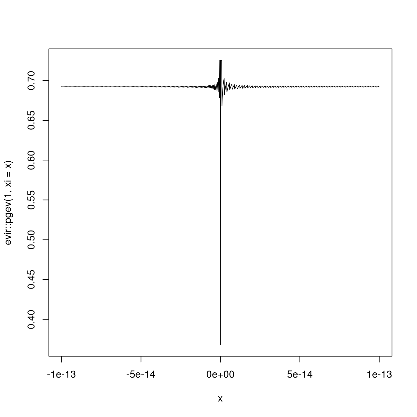
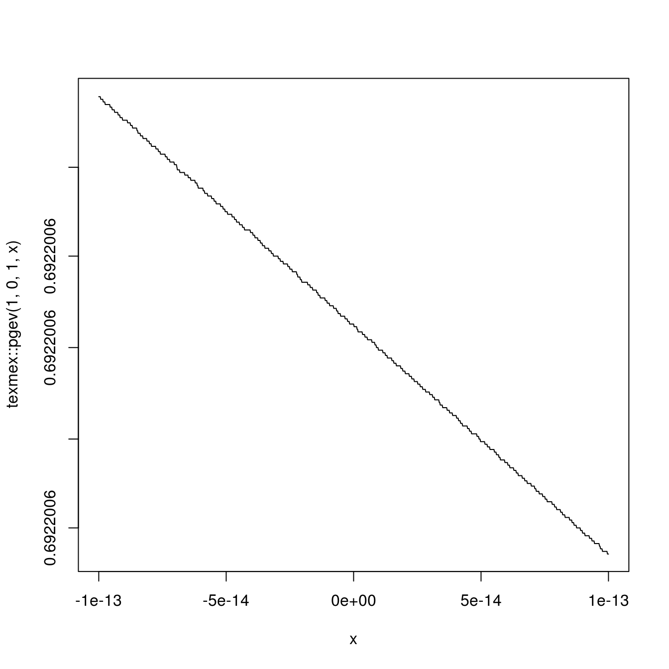
Figure 1.1: Two implementations of GEV distribution function when \(\xi\) is close to zero.
Figure 1.1 shows a comparison of evaluating the GEV distribution function at \(x = 1\) for \(\mu = 0\), \(\sigma = 1\), and a sequence of \(\xi\) values near zero using two implementations.
1.3 Exercises
Use git to clone the source of Hadley Wickham’s Advanced R Programming from his GitHub repository to a local space on your own computer. Build the book using RStudio. During the building process, you may see error messages due to missing tools on your computer. Read the error messages carefully and fix them, until you get the book built. You may need to install some R packages, some fonts, some latex packages, and some building tools for R packages. On Windows, some codes for parallel computing may not work and need to be swapped out. Document your computing environment (operating system, R/RStudio, Shell, etc.) and the problems you encountered, as well as how you solved them in an R Markdown file named
README.Rmd. Push it to your homework GitHub repository so that it can help other students to build the book.Use bookdown or rmarkdown to produce a report for the following task. Consider approximation of the distribution function of \(N(0, 1)\), \[\begin{equation} \Phi(t) = \int_{-\infty}^t \frac{1}{\sqrt{2\pi}} e^{-y^2 / 2} \mathrm{d}y, \tag{1.1} \end{equation}\] by the Monte Carlo methods: \[\begin{equation} \hat\Phi(t) = \frac{1}{n} \sum_{i=1}^n I(X_i \le t), \end{equation}\] where \(X_i\)’s are a random sample from \(N(0, 1)\), and \(I(\cdot)\) is the indicator function. Experiment with the approximation at \(n \in \{10^2, 10^3, 10^4\}\) at \(t \in \{0.0, 0.67, 0.84, 1.28, 1.65, 2.32, 2.58, 3.09, 3.72\}\) to form a table.
The table should include the true value for comparison. Further, repeat the experiment 100 times. Draw box plots of the 100 approximation errors at each \(t\) using ggplot2 (Wickham et al. 2020) for each \(n\). The report should look like a manuscript, with a title, an abstract, and multiple sections. It should contain at least one math equation, one table, one figure, and one chunk of R code. The template of our Data Science Lab can be helpful: https://statds.org/template/, the source of which is at https://github.com/statds/dslab-templates.
Explain how
.Machine$double.xmax,.Machine$double.xmin,.Machine$double.eps, and.Machine@double.neg.epsare defined using the 64-bit double precision floating point arithmetic. Give the 64-bit representation for these machine constants as well as the double precision number 1.0, 0.0, and \(\pi\).Find the first 10-digit prime number occurring in consecutive digits of \(e\) http://mathworld.wolfram.com/news/2004-10-13/google/. Hint: How can \(e\) be represented to an arbitrary precision?
1.4 Course Project
Each student is required to work independently on a class project on a topic of your choice that involves computing. Examples are an investigation of the properties of a methodology you find interesting, a comparison of several methods on a variety of problems, a comprehensive analysis of a real data with methodologies from the course, or an R package. The project should represent new work, not something you have done for another course or as part of your thesis. I have a collection of small problems that might be suitable. Projects from Kaggle data science competitions may be good choices too.
- Project proposal is due in week 7, the middle of the semester. This is a detailed, one-page description of what you plan to do, including question(s) to be addressed and models/methods to be used.
- Project interim report is due in week 12. This informal report will indicate that your project is ``on track’’. The report includes results obtained thus far and a brief summary of what they mean and what remains to be done. Students often start working on this too late. Your do not want to make the same mistake.
- Final project report is due in the exam week. The final form of the report should use the Data Science Lab template, of no more than 6 pages (single spaced, font no smaller than 11pt, 1 inch margin, with references, graphics and tables included).
- With more effort, a good project can turn into a paper and be submitted to ENAR student paper competition (Oct. 15) and ASA student paper competition (Dec. 15).
Project ideas:
- An animated demonstration of different methods in optimx with data examples.
- Accelerated EM algorithm
- Simulation from empirical distributions joined by copulas
References
Burns, Patrick. 2012. The R Inferno. Lulu. com.
Gillespie, Colin, and Robin Lovelace. 2016. Efficient R Programming: A Practical Guide to Smarter Programming. " O’Reilly Media, Inc.".
Gray, Robert. 2001. Advanced Statistical Computing.
Srivastava, Anuj. 2009. Computational Methods in Statistics.
Wickham, Hadley. 2019. Advanced R. 2nd ed. Chapman; Hall/CRC.
Wickham, Hadley, Winston Chang, Lionel Henry, Thomas Lin Pedersen, Kohske Takahashi, Claus Wilke, Kara Woo, Hiroaki Yutani, and Dewey Dunnington. 2020. Ggplot2: Create Elegant Data Visualisations Using the Grammar of Graphics. https://CRAN.R-project.org/package=ggplot2.
Xie, Yihui. 2016. bookdown: Authoring Books and Technical Documents with R Markdown. Boca Raton, Florida: Chapman; Hall/CRC. https://github.com/rstudio/bookdown.
Xie, Yihui, Amber Thomas, and Alison Presmanes Hill. 2017. blogdown: Creating Websites with R Markdown. Boca Raton, Florida: Chapman; Hall/CRC. https://github.com/rstudio/blogdown.