Chapter 3 Optimization

Recall the MLE example in Chapter 1. Consider a random sample \(X_1, \ldots, X_n\) of size \(n\) coming from a univariate distribution with density function \(f(x | \theta)\), where \(\theta\) is a parameter vector. The MLE \(\hat\theta_n\) of the unknown parameter \(\theta\) is obtained by maximizing the loglikelihood function \[ l(\theta) = \sum_{i=1}^n \log f(X_i | \theta) \] with respect to \(\theta\). Typically, \(\hat\theta\) is obtained by solving the score equation \[ l'(\theta) = \sum_{i=1}^n \frac{\partial}{\partial \theta} \log f(X_i; \theta) = 0, \] i.e., the derivative of the loglikelihood function equated to zero. From mathematical statistics, it is known that, under certain regularity conditions, \[\begin{align*} \mathbb{E}\frac{\partial}{\partial \theta} \log f(X; \theta) &= 0,\\ \mathbb{E}\frac{\partial}{\partial \theta} \log f(X; \theta) \left[\frac{\partial}{\partial \theta} \log f(X; \theta) \right]^{\top} &= - \mathbb{E} \frac{\partial^2}{\partial \theta \partial \theta^{\top}} \log f(X; \theta). \end{align*}\] The expectation in the second equation is known as the Fisher information \(I(\theta)\), a nonnegative definite matrix. Large sample results state that, as \(n \to \infty\), \(\hat\theta_n\) is consistent for \(\theta\) and \(\sqrt{n} (\hat\theta_n - \theta)\) converges in distribution to \(N(0, I^{-1}(\theta))\). The asymptotic variance of \(\hat\theta\) can be estimated by inverting the observed Fisher information matrix \(l''(\hat\theta_n)\).

More generally in Statistics, M-estimators are a broad class of extremum estimators obtained by maximizing an data dependent objective function. Both non-linear least squares and maximum likelihood estimation are special cases of M-estimators. The definition of M-estimators was motivated by robust statistics, which contributed new types of M-estimators. When the objective function is smooth, the M-estimator can be obtained by solving the corresponding “score” equation. Clearly, optimization or root-finding are very important in Statistics.

3.1 Univariate Optimizations

Optimization and root finding are closely related. Consider maximization of a smooth and differentiable function \(g(x)\). A necessary condition at the maximum is \(f(x) = g'(x) = 0\). Univariate illustrations help to gain insights about the ideas.

3.1.1 Bisection Method

The bisection method repeatedly bisects an interval and then selects a subinterval in which a root must lie for further processing. It is a very simple and robust method, but relatively slow.

The method is applicable for solving the equation \(f(x) = 0\) for the real variable \(x\), where \(f\) is a continuous function defined on an interval \([a, b]\) and \(f(a)\) and \(f(b)\) have opposite signs. This method is illustrated with an animation using the package animation (Xie 2018).

animation::bisection.method()

3.1.2 Newton’s Method

A fast approach to find roots of a differentiable function \(f(x)\). The methods starts from some initial value \(x_0\), and for \(t = 0, 1, \ldots\), compute \[\begin{align*} x_{t+1} = x_t - \frac{f(x_t)}{f'(x_t)} \end{align*}\] until \(x_t\) converges. The method is based on a linear expansion of \(f(x)\). The method is also known as Newton–Raphson iteration. It needs an initial value \(x_0\). If \(f(x) = 0\) has multiple solutions, the end result depends on \(x_0\).

Applied to optimization of \(g\), this method requires the Hessian \(g''\), which can be difficult to obtain, especially for multivariate functions. Many variants of Newton’s method avoid the computation of the Hessian.

For example, to obtain MLE with likelihood \(l(\theta)\), Fisher scoring replaces \(-l''(\theta_t)\) with \(I(\theta_t)\). Generally, one uses Fisher scoring in the beginning to make rapid improvements, and Newton’s method for refinement near the end.

The secant method approximates \(f'(x_t)\) by \[\begin{align*} \frac{f(x_t) - f(x_{t-1})}{x_t - x_{t-1}}. \end{align*}\] Given initial values \(x_0\) and \(x_1\), the iteration is \[\begin{align*} x_{t+1} = x_t - \frac{f(x_t)(x_t- x_{t-1})}{f(x_t) - f(x_{t-1})}. \end{align*}\]

3.1.3 Fixed Point Iteration

A fixed point of a function is a point whose evaluation by that function equals to itself, i.e., \(x = G(x)\).

Fixed point iteration: the natural way of hunting for a fixed point is to use \(x_{t+1} = G(x_t)\).

Definition 3.1 A function \(G\) is contractive on \([a,b]\) if \[\begin{align*} (1).\,\, & G(x)\in [a,b] \mbox{ whenever } x\in [a,b],\\ (2).\,\, & |G(x_1) - G(x_2)| \leq \lambda |x_1-x_2| \mbox{ for all } x_1,x_2\in [a,b] \mbox{ and some } \lambda\in [0,1). \end{align*}\]

Theorem 3.1 If \(G\) is contractive on \([a,b]\), then there is a unique fixed point \(x^*\in [a,b]\), and the fixed point iteration convergence to it when starting inside the interval.

Convergence: \(|x_{t+1}-x_{t}|=|G(x_t)-G(x_{t-1})|\leq \lambda |x_t - x_{t-1}|\leq \lambda^{t}|x_1-x_0| \rightarrow 0\), as \(t\rightarrow \infty\). It follows that \(\{x_t\}\) convergent to a limit \(x^*\).

Application in root finding: for solving \(f(x)=0\), we can simply let \(G(x) = x + \alpha f(x)\), where \(\alpha \neq 0\) is a constant.

Required Lipschitz condition: \(|x - y + \alpha [f(x) - f(y)]| \le \lambda|x-y|\), for some \(\lambda \in [0,1)\) and for all \(x,y\in [a,b]\). This holds if \(|G'(x)|\leq \lambda\) for some \(\lambda \in [0,1)\) and for all \(x\in [a,b]\), i.e., \(|1+\alpha f'(x)|\leq\lambda\). (use mean value theorem.)

Newton’s methods: \(G(x) = x - f(x)/f'(x)\). So it is as if \(\alpha_t\) is chosen adaptively as \(\alpha_t=-1/f'(x_t)\). This leads to a faster convergence order (quadratic).

3.2 Multivariate Optimization

Consider maximizing a real-valued objective function \(g(x)\) of \(p\)-dimensional vector \(x\).

3.2.1 Newton-Raphson Method

The Newton-Raphson method is a generalization of univariate Newton’s root finding algorithm to the multivariate case.

3.2.2 Variants of Newton-Raphson Method

The motivation is to avoid the calculation of the Hessian matrix in updatings with the form \[ x^{(t + 1)} = x^{(t)} - (M^{(t)})^{-1} g'(x), \] where \(g'\) is the gradient of \(g\) and \(M\) is a substitute of \(g''(x)\).

3.2.2.1 Fisher Scoring

Choose \(M\) as the negative Fisher information matrix. For location-families, it can be shown that the information matrix is free of the location parameter.

3.2.2.2 Steepest Ascent

Choose \(M = \alpha^{(t)} I_p\) for \(\alpha^{(t)} > 0\) so the updating in the direction of he steepest ascent.

3.2.2.3 Discrete Newton

Approximate the Hessian matrix with finite-difference quotients.

3.2.2.4 Fixed-Point Iteration

Choose \(M^{(t)} = M\) for all \(t\). An example is \(M = g''(x_0)\).

3.2.2.5 Quasi-Newton

Quasi-Newton methods avoids Hessian matrix by constructing approximations of the inverse Hessian. The inverse Hessian is built up from gradient information obtained at various points.

Rank-two update. The celebrated BFGS is a rank-two update method. Box constraints can be allowed with L-BFGS-B.

3.2.2.6 Coordinate Descent

Coordinate descent algorithms optimize a objective function with respect to a single parameter or a block of parameters at a time, iteratively cycling through all parameters until convergence is reached. How to determine the blocks of parameters is problem-specific. The method is ideal for problems that have a simple closed form solution in a single/lower dimension but lack one in higher dimensions. % The method is also called backfitting or Gauss–Seidel iteration. It is very commonly used in fitting penalized regression. The concept also appears in many well-known estimation problems. The simple technique can be surprisingly efficient and scalable.

Consider objective function \[ f(\beta) = g(\beta) + \sum_{j=1}^{p}h_j(\beta_j), \] where \(g\) is convex and differentiable and each \(h_i\) is convex. The second part is usually non-smooth, but is separable. Coordinate descent start with some initial guess \(\beta^{(0)}\), repeat the following for \(k=1,2,3...\): \[\begin{align*} \beta_1^{(k)} & = \arg\min_{\beta_1}f(\beta_1,\beta_2^{(k-1)},\ldots,\beta_p^{(k-1)}),\\ \beta_2^{(k)} & = \arg\min_{\beta_2}f(\beta_1^{(k)},\beta_2, \beta_3^{(k-1)},\ldots,\beta_p^{(k-1)}),\\ & \ldots\\ \beta_p^{(k)} & = \arg\min_{\beta_p}f(\beta_1^{(k)},\ldots,\beta_{p-1}^{(k)},\beta_p). \end{align*}\] It can be shown that if we are at a point \(\beta\) such that \(f(\beta)\) is minimized along each coordinate axis, we have found a global minimizer.

Remarks:

• Order of cycle through coordinates is arbitrary.
• Can replace individual coordinates with blocks of coordinates.
• Same idea has been applied to many non-convex problems.
• As long as the objective function is monotone decreasing, the convergence is guaranteed.

3.2.2.7 Conjugate Gradient

3.2.2.8 Gauss-Newton

Non-linear least squares.

3.2.3 Nelder-Mead (Simplex) Algorithm

Not even the gradient is needed. Possible moves are: reflection; expansion; outer contraction; inner contraction; shrinkage.

Consider minimizing this simple function.

f1 <- function(x) {
  x1 <- x[1]
  x2 <- x[2]
  x1^2 + 3*x2^2  
}

Apparently the minimizer is \((0, 0)\). Let’s track all the points at which the function is evaluated in the Nelder-Mead algorithm.

trace(f1, exit = quote(print(c(returnValue(), x))))

## [1] "f1"

optim(c(1, 1), f1, control = list(trace = TRUE))

##   Nelder-Mead direct search function minimizer
## Tracing fn(par, ...) on exit 
## [1] 4 1 1
## function value for initial parameters = 4.000000
##   Scaled convergence tolerance is 5.96046e-08
## Stepsize computed as 0.100000
## Tracing fn(par, ...) on exit 
## [1] 4.21 1.10 1.00
## Tracing fn(par, ...) on exit 
## [1] 4.63 1.00 1.10
## BUILD              3 4.630000 4.000000
## Tracing fn(par, ...) on exit 
## [1] 3.64 1.10 0.90
## Tracing fn(par, ...) on exit 
## [1] 3.2425 1.1500 0.8000
## EXTENSION          5 4.210000 3.242500
## Tracing fn(par, ...) on exit 
## [1] 3.0225 1.0500 0.8000
## Tracing fn(par, ...) on exit 
## [1] 2.520625 1.025000 0.700000
## EXTENSION          7 4.000000 2.520625
## Tracing fn(par, ...) on exit 
## [1] 2.130625 1.175000 0.500000
## Tracing fn(par, ...) on exit 
## [1] 1.781406 1.262500 0.250000
## EXTENSION          9 3.242500 1.781406
## Tracing fn(par, ...) on exit 
## [1] 1.361406 1.137500 0.150000
## Tracing fn(par, ...) on exit 
## [1]  1.371602  1.131250 -0.175000
## REFLECTION        11 2.520625 1.361406
## Tracing fn(par, ...) on exit 
## [1]  2.160625  1.375000 -0.300000
## Tracing fn(par, ...) on exit 
## [1]  1.665156  1.287500 -0.050000
## LO-REDUCTION      13 1.781406 1.361406
## Tracing fn(par, ...) on exit 
## [1]  1.418906  1.162500 -0.150000
## Tracing fn(par, ...) on exit 
## [1]  1.417656  1.187500 -0.050000
## LO-REDUCTION      15 1.665156 1.361406
## Tracing fn(par, ...) on exit 
## [1] 1.143906 1.037500 0.150000
## Tracing fn(par, ...) on exit 
## [1] 1.020156 0.912500 0.250000
## EXTENSION         17 1.417656 1.020156
## Tracing fn(par, ...) on exit 
## [1] 1.351406 0.862500 0.450000
## Tracing fn(par, ...) on exit 
## [1] 1.207539 0.943750 0.325000
## LO-REDUCTION      19 1.361406 1.020156
## Tracing fn(par, ...) on exit 
## [1] 1.058477 0.718750 0.425000
## Tracing fn(par, ...) on exit 
## [1] 1.0587915 0.8234375 0.3562500
## LO-REDUCTION      21 1.207539 1.020156
## Tracing fn(par, ...) on exit 
## [1] 0.8401563 0.6875000 0.3500000
## Tracing fn(par, ...) on exit 
## [1] 0.7071191 0.5593750 0.3625000
## EXTENSION         23 1.058477 0.707119
## Tracing fn(par, ...) on exit 
## [1] 0.672666 0.753125 0.187500
## Tracing fn(par, ...) on exit 
## [1] 0.6075610 0.7703125 0.0687500
## EXTENSION         25 1.020156 0.607561
## Tracing fn(par, ...) on exit 
## [1] 0.2726001 0.4171875 0.1812500
## Tracing fn(par, ...) on exit 
## [1] 0.09345764 0.16953125 0.14687500
## EXTENSION         27 0.707119 0.093458
## Tracing fn(par, ...) on exit 
## [1]  0.2094733  0.3804688 -0.1468750
## Tracing fn(par, ...) on exit 
## [1]  0.18193546  0.42519531 -0.01953125
## LO-REDUCTION      29 0.607561 0.093458
## Tracing fn(par, ...) on exit 
## [1]  0.04113010 -0.17558594  0.05859375
## Tracing fn(par, ...) on exit 
## [1]  0.42918962 -0.64853516  0.05351562
## REFLECTION        31 0.181935 0.041130
## Tracing fn(par, ...) on exit 
## [1]  0.3378516 -0.4312500  0.2250000
## Tracing fn(par, ...) on exit 
## [1] 0.04974852 0.21108398 0.04160156
## HI-REDUCTION      33 0.093458 0.041130
## Tracing fn(par, ...) on exit 
## [1]  0.02450188 -0.13403320 -0.04667969
## Tracing fn(par, ...) on exit 
## [1]  0.1434302 -0.2858154 -0.1434570
## REFLECTION        35 0.049749 0.024502
## Tracing fn(par, ...) on exit 
## [1]  0.2737758 -0.5207031 -0.0296875
## Tracing fn(par, ...) on exit 
## [1] 0.002488067 0.028137207 0.023779297
## HI-REDUCTION      37 0.041130 0.002488
## Tracing fn(par, ...) on exit 
## [1]  0.02478057  0.06968994 -0.08149414
## Tracing fn(par, ...) on exit 
## [1]  0.006549060  0.008370972 -0.046472168
## LO-REDUCTION      39 0.024502 0.002488
## Tracing fn(par, ...) on exit 
## [1] 0.03081047 0.17054138 0.02398682
## Tracing fn(par, ...) on exit 
## [1]  0.005876474 -0.057889557 -0.029013062
## HI-REDUCTION      41 0.006549 0.002488
## Tracing fn(par, ...) on exit 
## [1]  0.006555205 -0.038123322  0.041238403
## Tracing fn(par, ...) on exit 
## [1]  0.001817881 -0.003252602 -0.024544525
## HI-REDUCTION      43 0.005876 0.001818
## Tracing fn(par, ...) on exit 
## [1] 0.009245382 0.082774162 0.028247833
## Tracing fn(par, ...) on exit 
## [1]  0.001164443 -0.022723627 -0.014697838
## HI-REDUCTION      45 0.002488 0.001164
## Tracing fn(par, ...) on exit 
## [1]  0.01484345 -0.05411344 -0.06302166
## Tracing fn(par, ...) on exit 
## [1] 7.034119e-05 7.574546e-03 2.079058e-03
## HI-REDUCTION      47 0.001818 0.000070
## Tracing fn(par, ...) on exit 
## [1]  0.0005681964 -0.0118964791  0.0119257450
## Tracing fn(par, ...) on exit 
## [1]  0.0001184377 -0.0097355098  0.0028081775
## LO-REDUCTION      49 0.001164 0.000070
## Tracing fn(par, ...) on exit 
## [1] 0.001573548 0.020562664 0.019585073
## Tracing fn(par, ...) on exit 
## [1]  0.0002542833 -0.0119020544 -0.0061271101
## HI-REDUCTION      51 0.000254 0.000070
## Tracing fn(par, ...) on exit 
## [1] 0.0004588363 0.0097410910 0.0110143453
## Tracing fn(par, ...) on exit 
## [1]  5.231265e-05 -6.491268e-03 -1.841746e-03
## HI-REDUCTION      53 0.000118 0.000052
## Tracing fn(par, ...) on exit 
## [1]  0.0001368742  0.0108187880 -0.0025708660
## Tracing fn(par, ...) on exit 
## [1]  2.755658e-05 -4.596935e-03  1.463417e-03
## HI-REDUCTION      55 0.000070 0.000028
## Tracing fn(par, ...) on exit 
## [1]  0.0003664145 -0.0186627497 -0.0024573874
## Tracing fn(par, ...) on exit 
## [1] 3.709448e-06 1.015222e-03 9.449464e-04
## HI-REDUCTION      57 0.000052 0.000004
## Tracing fn(par, ...) on exit 
## [1] 0.0000626558 0.0029095551 0.0042501093
## Tracing fn(par, ...) on exit 
## [1]  1.745326e-05 -4.141062e-03 -3.187824e-04
## HI-REDUCTION      59 0.000028 0.000004
## Tracing fn(par, ...) on exit 
## [1]  4.267097e-06  1.471095e-03 -8.372525e-04
## Tracing fn(par, ...) on exit 
## [1]  2.081740e-07 -4.591230e-05 -2.620853e-04
## LO-REDUCTION      61 0.000017 0.000000
## Tracing fn(par, ...) on exit 
## [1] 2.912577e-05 5.110372e-03 1.001644e-03
## Tracing fn(par, ...) on exit 
## [1]  3.342713e-06 -1.828204e-03  1.132410e-05
## HI-REDUCTION      63 0.000004 0.000000
## Tracing fn(par, ...) on exit 
## [1]  1.263743e-05 -2.889338e-03 -1.195708e-03
## Tracing fn(par, ...) on exit 
## [1] 5.052935e-07 3.908218e-05 4.097829e-04
## HI-REDUCTION      65 0.000003 0.000000
## Tracing fn(par, ...) on exit 
## [1] 3.373195e-06 1.821374e-03 1.363736e-04
## Tracing fn(par, ...) on exit 
## [1]  8.441476e-07 -9.158093e-04  4.258647e-05
## HI-REDUCTION      67 0.000001 0.000000
## Tracing fn(par, ...) on exit 
## [1] 8.593883e-07 9.089792e-04 1.051112e-04
## Tracing fn(par, ...) on exit 
## [1]  2.214113e-07 -4.596122e-04  5.821765e-05
## HI-REDUCTION      69 0.000001 0.000000
## Tracing fn(par, ...) on exit 
## [1]  1.426297e-06 -5.446067e-04 -6.136505e-04
## Tracing fn(par, ...) on exit 
## [1]  8.249310e-08 -1.068400e-04  1.539246e-04
## HI-REDUCTION      71 0.000000 0.000000
## Tracing fn(par, ...) on exit 
## [1]  1.772082e-07  3.068599e-04 -1.663784e-04
## Tracing fn(par, ...) on exit 
## [1]  4.973221e-08  1.152418e-04 -1.102294e-04
## LO-REDUCTION      73 0.000000 0.000000
## Tracing fn(par, ...) on exit 
## [1] 2.834551e-07 5.431411e-05 3.057805e-04
## Tracing fn(par, ...) on exit 
## [1]  4.372056e-08 -2.085570e-05 -1.201188e-04
## Exiting from Nelder Mead minimizer
##     75 function evaluations used

## $par
## [1] -0.0000208557 -0.0001201188
## 
## $value
## [1] 4.372056e-08
## 
## $counts
## function gradient 
##       75       NA 
## 
## $convergence
## [1] 0
## 
## $message
## NULL

untrace(f1)

It is possible that the Nelder–Mead algorithm converges to points that are not local optima. See Example 2.9 in the GH book.

Questions: 1. How is the initial simplex constructed? 2. How to set the stopping criteria?

Advanced methods are available in R package .

3.2.4 Optimization with R

See conversation with John Nash about r optim and r optimx.

3.3 MM Algorithm

The MM algorithm may be viewed as philosophy for optimization algorithms. The EM algorithm is a special case. An MM algorithm operates by creating a surrogate function that majorizes (minorizes) the objective function. When the surrogate function is optimized, the objective function is driven downhill (uphill). The MM can stand for majorization-minimization or minorization-maximization. The algorithm may avoid matrix inversion, linearize an optimization problem, conveniently deal with equality and inequality constraints, and solve a non-differentiable problem by iteratively solving smooth problems.

A function \(g(\theta \mid \theta^s)\) is said to majorize the function \(f(\theta)\) at \(\theta^s\) if \[ f(\theta^s) = g(\theta^s \mid \theta^s), \] and \[ f(\theta) \leq g(\theta \mid \theta^s) \] for all \(\theta\).

The descent property of the MM algorithm is easy to see. Let \[ \theta^{s+1} = \arg\min_\theta g(\theta \mid \theta^s). \] It follows that \[\begin{align*} f(\theta^{s+1}) \leq g(\theta^{s+1} \mid \theta^s) \leq g(\theta^{s} \mid \theta^s) = f(\theta^s). \end{align*}\] The strict inequality holds unless \(g(\theta^{s+1} \mid \theta^s)=g(\theta^{s} \mid \theta^s)\) and \(f(\theta^{s+1})= g(\theta^{s+1} \mid \theta^s)\). Therefore, by alternating between the majorization and the minimization steps, the objective function is monotonically decreasing and thus its convergence is guaranteed.

par(mar=c(2.5, 2.5, 0.1, 0.1), mgp=c(1.5, 0.5, 0))
f <- function(x) abs(x - 1) + abs(x - 3) + abs(x - 4) + abs(x - 8) + abs(x - 10)
curve(f(x), 0, 12)
g <- function(x) (x - 5.5)^2 + 15.75
curve(g(x), 0, 12, add = TRUE, col="blue")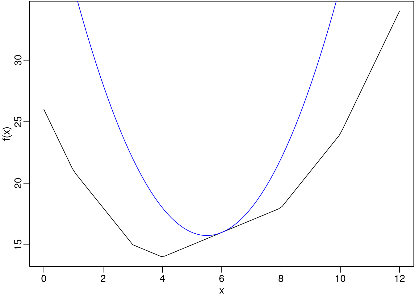

Inequalities are used to devise MM algorithms.

• Jensen’s inequality: for a convex function \(f(x)\), \[ f(E(X)) \leq E(f(X)). \]
• Convexity inequality: for any \(\lambda \in [0,1]\), \[ f(\lambda x_1 + (1-\lambda)x_2) \leq \lambda f(x_1) + (1-\lambda)f(x_2). \]
• Cauchy-Schwarz inequality.
• Supporting hyperplanes.
• Arithmetic-Geometric Mean Inequality.

3.4 An Example: LASSO with Coordinate Descent

In a linear regression setting, where \(Y\) is the response vector and \(X\) is the design matrix. Minimize objective function \[ \min_{\beta \in R^p}\left\{\frac{1}{2n}\|Y - X \beta\|^2 + \sum_{j = 1}^p p_{\lambda}(|\beta_j|)\right\}, \] where \(\|\cdot\|\) denotes the \(L_2\)-norm, and \(p_{\lambda}(\cdot)\) is a penalty function indexed by the regularization parameter \(\lambda \geq 0\). It is often assumed that the covariates are centered and standardized such that the coefficients become comparable.

Common penalties:

• \(L_0\) penalty (subset selection) and \(L_2\) penalty (ridge regression).
• Bridge or \(L_\gamma\) penalty, \(\gamma >0\)
• \(L_1\) penalty or Lasso
• SCAD penalty
• MCP penalty
• Group penalties
• Bilevel penalties

LASSO stands for ``least absolute shrinkage and selection operator’’. There are two equivalent definitions.

• minimize the residual sum of squares subject to the sum of the absolute value of the coefficients being less than a constant: \[ \hat{\beta}=\arg\min\left\{\frac{1}{2n}\|Y- X \beta\|^2\right\} \text{ subject to } \sum_{j}|\beta_j| \leq t. \]
• minimize the penalized sum of squares: \[ \hat{\beta}=\arg\min\left\{\frac{1}{2n}\|Y- X\beta\|^2 + \lambda\sum_{j}|\beta_j|\right\}. \]

Because of the nature of \(L_1\) penalty or constraint, Lasso can estimate some coefficients as exactly \(0\) and hence performs variable selection. It enjoys some of the favorable properties of both subset selection and ridge regression, producing interpretable models and exhibiting the stability of ridge regression.

A solution path for \(\lambda\in[\lambda_{\min},\lambda_{\max}]\) is \[ \{\widehat{\beta}_{n}(\lambda): \lambda\in[\lambda_{\min},\lambda_{\max}]\}. \]

For a given \(\lambda\), the coordinate descent algorithm minimize the objective function with respect to \(\beta_j\) given current values of \(\tilde\beta_k\), \(k \ne j\). Define \[ L_j(\beta_j; \lambda) = \frac{1}{2n}\sum_{i=1}^n \left(y_i - \sum_{k\ne j} x_{ik}\tilde\beta_k - x_{ij} \beta_j\right)^2 + \lambda |\beta_j|. \] Let \(\tilde y_{ij} = \sum_{k\ne j} x_{ik}\tilde\beta_k\), \(\tilde r_{ij} = y_i - \tilde y_{ij}\), and \(\tilde z_j = n^{-1} \sum_{i=1}^n x_{ij} \tilde r_{ij}\). Note that \(\tilde r_{ij}\)’s are the partial residual with respect to the \(j\)th covariate. Assuming that the covariates are centered and standardized such that \(\sum_{i=1}^{n}x_{ij}=0\) and \(\sum_{i=1}^{n}x_{ij}^2=n\) for all \(1\leq j \leq p\), the standardized covariates and completion of squares lead to

\[ L_j(\beta_j; \lambda) = \frac{1}{2}(\beta_j - \tilde z_j)^2 + \lambda |\beta_j| + \frac{1}{2n} \sum_{i=1}^n \tilde r_{ij}^2 - \frac{1}{2} \tilde z_j^2. \] This is just a univariate quadratic programming problem. The solution is \[ \tilde \beta_j = S(\tilde z_{j}; \lambda) \] where \(S(\cdot; \lambda)\) is the soft-threshold operator \[ S(z; \lambda) = \mathrm{sgn}(z) (|z| - \lambda)_+ = \begin{cases} z - \lambda, & z > \lambda,\\ 0, & |z| \le \lambda,\\ z + \lambda, & z < -\lambda.\\ \end{cases} \]

The last question is, how do we choose \(\lambda\)? Cross-validation or generalized cross-validation.

3.5 Exercises

3.5.1 Cauchy with unknown location.

Consider estimating the location parameter of a Cauchy distribution with a known scale parameter. The density function is \[\begin{align*} f(x; \theta) = \frac{1}{\pi[1 + (x - \theta)^2]}, \quad x \in R, \quad \theta \in R. \end{align*}\] Let \(X_1, \ldots, X_n\) be a random sample of size \(n\) and \(\ell(\theta)\) the log-likelihood function of \(\theta\) based on the sample.

1. Show that \[\begin{align*} \ell(\theta) &= -n\ln \pi - \sum_{i=1}^n \ln [1+(\theta-X_i)^2], \\ \ell'(\theta) &= -2 \sum_{i=1}^n \frac{\theta-X_i}{1+(\theta-X_i)^2}, \\ \ell''(\theta) &= -2 \sum_{i=1}^n \frac{1-(\theta-X_i)^2}{[1+(\theta-X_i)^2]^2}, \\ I_n(\theta) &= \frac{4n}{\pi} \int_{-\infty}^\infty \frac{x^2\,\mathrm{d}x}{(1+x^2)^3} = n/2, \end{align*}\] where \(I_n\) is the Fisher information of this sample.
2. Set the random seed as \(909\) and generate a random sample of size \(n = 10\) with \(\theta = 5\). Implement a loglikelihood function and plot against \(\theta\).
3. Find the MLE of \(\theta\) using the Newton–Raphson method with initial values on a grid starting from \(-10\) to \(30\) with increment \(0.5\). Summarize the results.
4. Improved the Newton–Raphson method by halving the steps if the likelihood is not improved.
5. Apply fixed-point iterations using \(G(\theta)=\alpha \ell'(\theta) + \theta\), with scaling choices of \(\alpha \in \{1, 0.64, 0.25\}\) and the same initial values as above.
6. First use Fisher scoring to find the MLE for \(\theta\), then refine the estimate by running Newton-Raphson method. Try the same starting points as above.
7. Comment on the results from different methods (speed, stability, etc.).

3.5.2 Many local maxima

Consider the probability density function with parameter \(\theta\): \[\begin{align*} f(x; \theta) = \frac{1 - \cos(x - \theta)}{2\pi}, \quad 0\le x\le 2\pi, \quad \theta \in (-\pi, \pi). \end{align*}\] A random sample from the distribution is

x <- c(3.91, 4.85, 2.28, 4.06, 3.70, 4.04, 5.46, 3.53, 2.28, 1.96,
       2.53, 3.88, 2.22, 3.47, 4.82, 2.46, 2.99, 2.54, 0.52)

1. Find the the log-likelihood function of \(\theta\) based on the sample and plot it between \(-\pi\) and \(\pi\).
2. Find the method-of-moments estimator of \(\theta\). That is, the estimator \(\tilde\theta_n\) is value of \(\theta\) with \[\begin{align*} \mathbb{E}(X \mid \theta) = \bar X_n, \end{align*}\] where \(\bar X_n\) is the sample mean. This means you have to first find the expression for \(\mathbb{E}(X \mid \theta)\).
3. Find the MLE for \(\theta\) using the Newton–Raphson method initial value \(\theta_0 = \tilde\theta_n\).
4. What solutions do you find when you start at \(\theta_0 = -2.7\) and \(\theta_0 = 2.7\)?
5. Repeat the above using 200 equally spaced starting values between \(-\pi\) and \(\pi\). Partition the values into sets of attraction. That is, divide the set of starting values into separate groups, with each group corresponding to a separate unique outcome of the optimization.

3.5.3 Modeling beetle data

The counts of a floor beetle at various time points (in days) are given in a dataset.

beetles <- data.frame(
    days    = c(0,  8,  28,  41,  63,  69,   97, 117,  135,  154),
    beetles = c(2, 47, 192, 256, 768, 896, 1120, 896, 1184, 1024))

A simple model for population growth is the logistic model given by \[ \frac{\mathrm{d}N}{\mathrm{d}t} = r N(1 - \frac{N}{K}), \] where \(N\) is the population size, \(t\) is time, \(r\) is an unknown growth rate parameter, and \(K\) is an unknown parameter that represents the population carrying capacity of the environment. The solution to the differential equation is given by \[ N_t = f(t) = \frac{K N_0}{N_0 + (K - N_0)\exp(-rt)}, \] where \(N_t\) denotes the population size at time \(t\).

• Fit the population growth model to the beetles data using the Gauss-Newton approach, to minimize the sum of squared errors between model predictions and observed counts.
• Show the contour plot of the sum of squared errors.
• In many population modeling application, an assumption of lognormality is adopted. That is , we assume that \(\log N_t\) are independent and normally distributed with mean \(\log f(t)\) and variance \(\sigma^2\). Find the maximum likelihood estimators of \(\theta = (r, K, \sigma^2)\) using any suitable method of your choice. Estimate the variance your parameter estimates.

3.5.4 Coordinate descent for penalized least squares

Consider the penalized least squares problem with \(L_1\) penalty (LASSO).

• Verify the soft-threshold solution.
• Find \(\lambda_{\max}\) such that for any \(\lambda > \lambda_\max\), the solution is \(\beta = 0\).
• Write a function to implement the soft-threshold solution for a given input z and lambda.
• Write a function pen_ls to implement the coordinate descent method for LASSO solution. The inputs of the function should include a response vector y, a model matrix xmat (with pre-standardized columns), and a penalty parameter lambda. The output is a vector of estimated \(\beta\).
• Test your pen_ls on a simulated dataset generated for a fixed \(\lambda\).

gen_data <- function(n, b, sigma = 1) {
  p <- length(b)
  x <- matrix(rnorm(n * p), n, p)
  colnames(x) <- paste0("x", 1:p)
  y <- c(x %*% b) + rnorm(n, sd = sigma)
  return(data.frame(y, x))
}

n <- 200
b <- c(1, -1, 2, rep(0, 7))
set.seed(920)
dat <- gen_data(n, b)

• Plot a solution path for a sequence of \(\lambda\) values from \(\lambda_\max\) to zero.

References

Xie, Yihui. 2018. Animation: A Gallery of Animations in Statistics and Utilities to Create Animations. https://yihui.name/animation.