Chapter 6 Markov Chain Monte Carlo

6.1 Eample: Normal mixture

Generate some data with mixing rate \(\delta\).

delta <- 0.7 # true value to be estimated based on the data
n <- 100
set.seed(123)
u <- rbinom(n, prob = delta, size = 1)
x <- rnorm(n, ifelse(u == 1, 7, 10), 0.5)

Assuming that the normal distribution parameters \(\mu_1\), \(\sigma_1^2\), \(\mu_2\), and \(\sigma_2^2\) are known. The only unknown parameter is \(\delta\). The likelihood function of \(\delta\) is

mylike <- function(delta, x) {
    prod(delta * dnorm(x, 7, 0.5) + (1 - delta) * dnorm(x, 10, 0.5))
}

We impose an uninformative prior on \(\delta\) and use a simple random walk proposal to construct the Metropolis–Hasting algorithm.

## simple random walk chain
myRange <- function(v, width) {
    min(1, v + width) - max(0, v - width)
}

mymcmc <- function(niter, init, x, width) {
    v <- double(niter)
    for (i in 1:niter) {
        cand <- runif(1, max(0, init - width), min(1, init + width))
        ratio <- mylike(cand, x) / myRange(cand, width) /
            mylike(init, x) * myRange(init, width)
        if (runif(1) < min(ratio, 1)) {
            v[i] <- init <- cand
        } else v[i] <- init
    }
    v
}

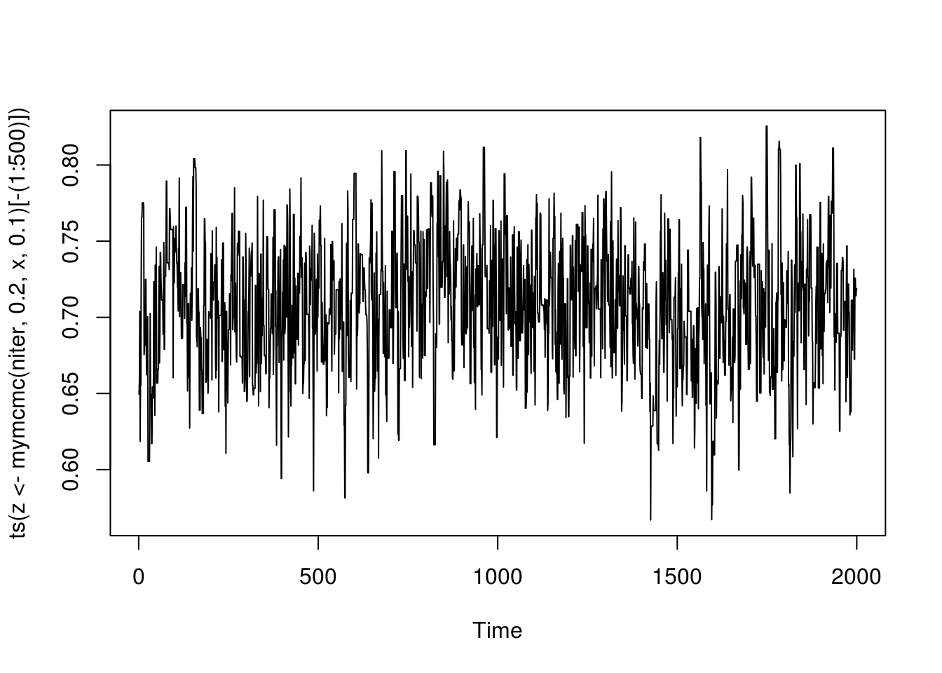
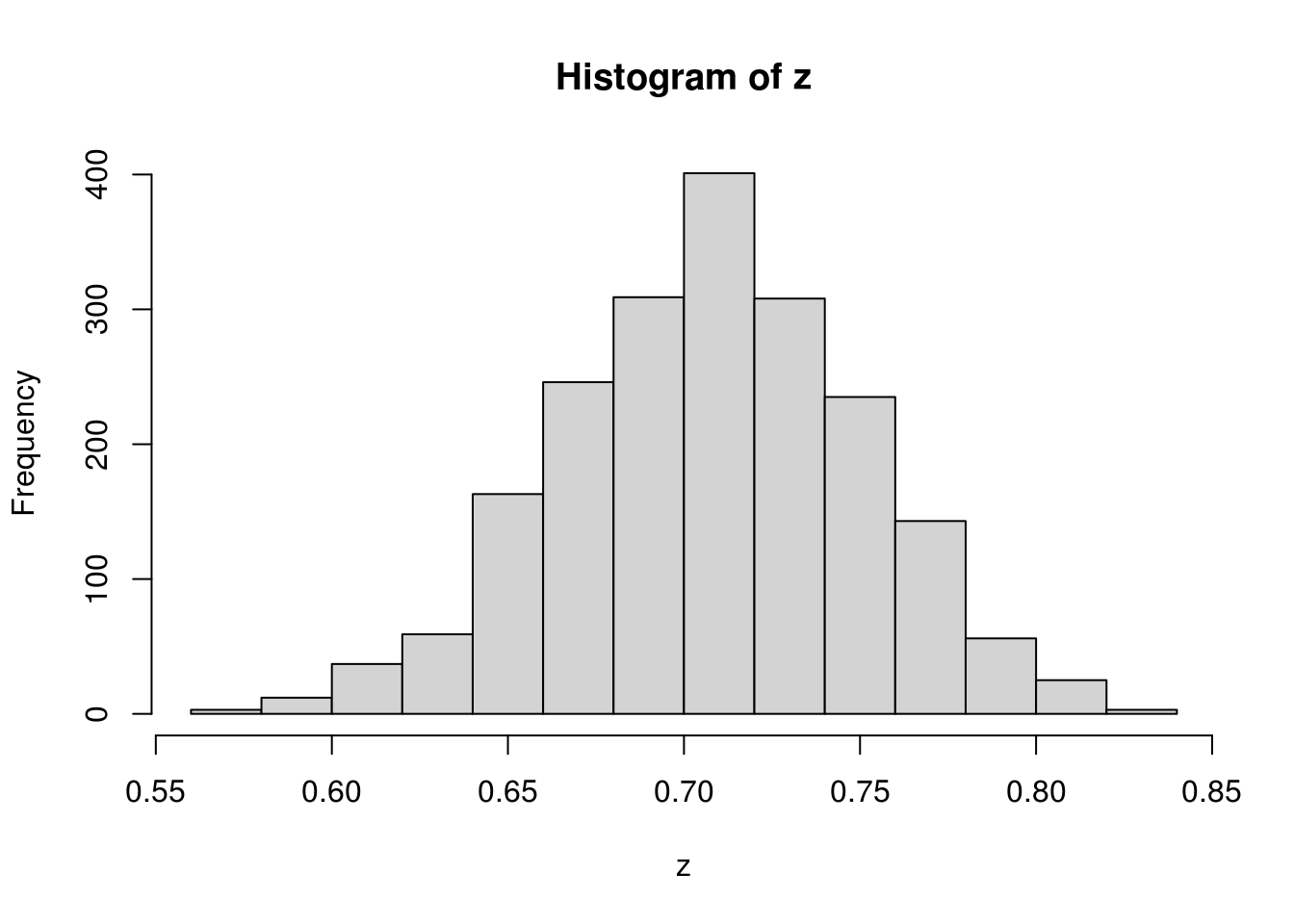
With initial value \(\delta_0 = .2\) and stepsize \(.1\) in the random walk proposal, we run the 2500 iterations and throw away the first 500 iterations.

niter <- 2500
plot(ts(z <- mymcmc(niter, .2, x, .1)[-(1:500)]))

hist(z)

6.2 General-Purpose Gibbs Sampling with the ARMS

Consider an example of posterior inference. Suppose that \((Y_i, X_i)\), \(i = 1, \ldots, n\), are observed, where \[ Y_i \mid X_i \sim \mbox{Poisson}(\exp(a + b X_i)). \] This is a Poisson regression model. Assume independent prior distributions on \(a\) and \(b\) with \(N(0, \sigma^2)\) and \(N(0, \tau^2)\). The posterior density of \((a, b)\) is \[ q(a, b \mid \mbox{data}) \propto \exp\left(a \sum_i^n Y_i + b \sum_i^n X_i Y_i - e^a \sum_i^n e^{X_i b} - \frac{a^2}{2\sigma^2} - \frac{b^2}{2\tau^2}\right). \] The full conditional distributions of \(a\) and \(b\) can be shown to be log-concave, which allows adaptive rejection alogorithm (Robert and Casella 2004). One could also just use the general ARMS as a lazy man’s approach.

Let us first generate some data.

n <- 100
a <- 0.0; b <- 0.5
x <- rnorm(n)
y <- rpois(n, exp(a + b * x))
mydata <- data.frame(y = y, x = x)

The posterior density up to an unknown normalizing constant can be easily computed.

logpost <- function(theta, data, sigma2, tau2) {
  a <- theta[1]; b <- theta[2]
  x <- data$x; y <- data$y
  return(a * sum(y) + b * sum(x * y) - exp(a) * sum(exp(b * x))
         - a^2 / 2 / sigma2 - b^2 / 2 / tau2)
}

An MCMC based the Gibbs sampler uses the ARMS algorithm from R package HI.

mymcmc <- function(niter, thetaInit, data, sigma2, tau2, nburn= 100) {
  p <- length(thetaInit)
  thetaCurrent <- thetaInit
  ## define a function for full conditional sampling  
  logFC <- function(th, idx) {
    theta <- thetaCurrent
    theta[idx] <- th
    logpost(theta, data, sigma2, tau2)
  }
  out <- matrix(thetaInit, niter, p, byrow = TRUE)
  ## Gibbs sampling
  for (i in 2:niter) {
    for (j in 1:p) {
      ## general-purpose arms algorithm
      out[i, j] <- thetaCurrent[j] <-
          HI::arms(thetaCurrent[j], logFC,
                   function(x, idx) ((x > -10) * (x < 10)), 
                   1, idx = j)
    }
  }
  out[-(1:nburn), ]
}

Now give it a try with \(\sigma^2 = 100\) and \(\tau^2 = 100\).

niter <- 600; nburn <- 100
thetaInit <- c(2, 2)
sigma2 <- tau2 <- 100
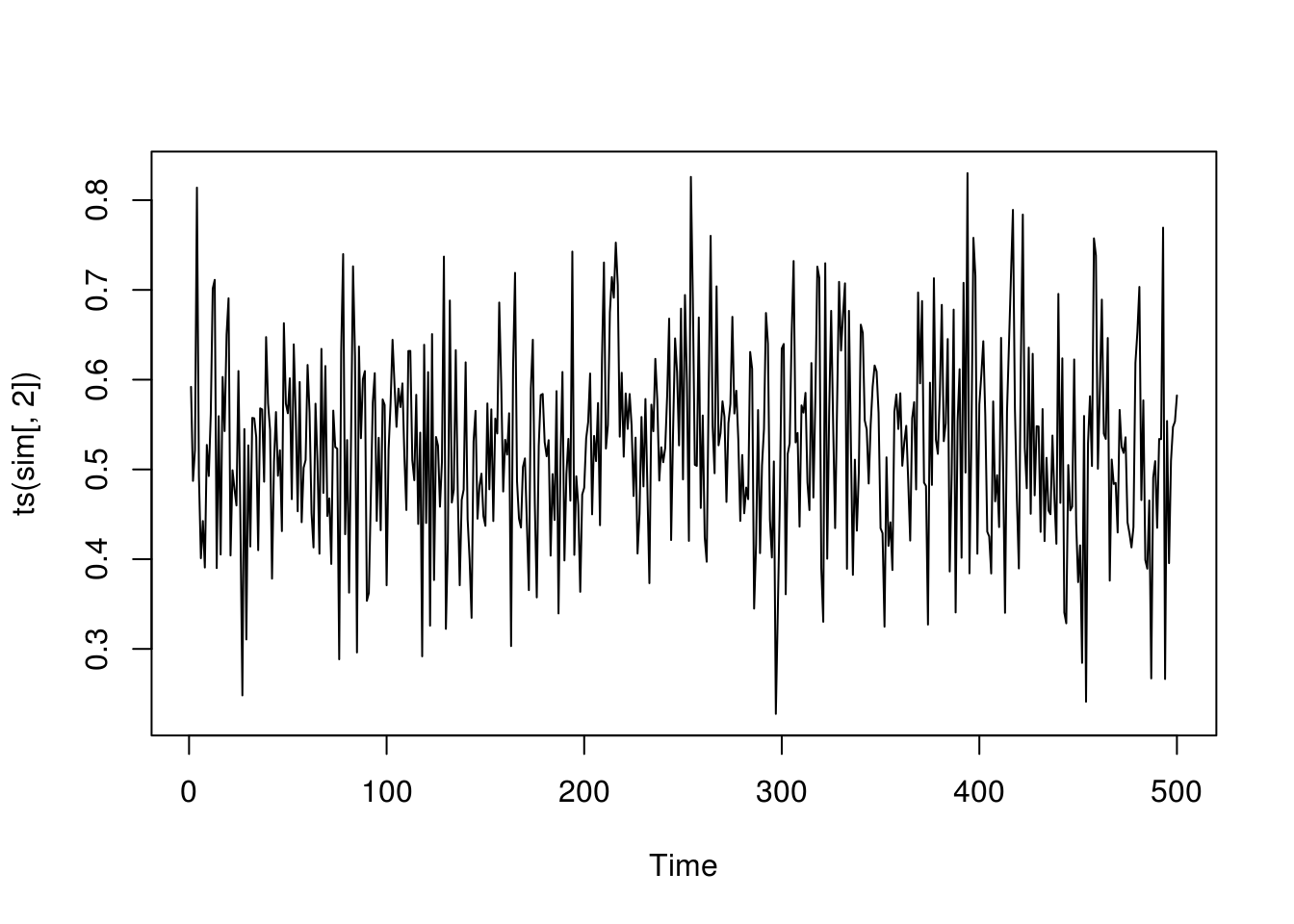
sim <- mymcmc(niter, thetaInit, mydata, sigma2, tau2)
plot(ts(sim[,1]))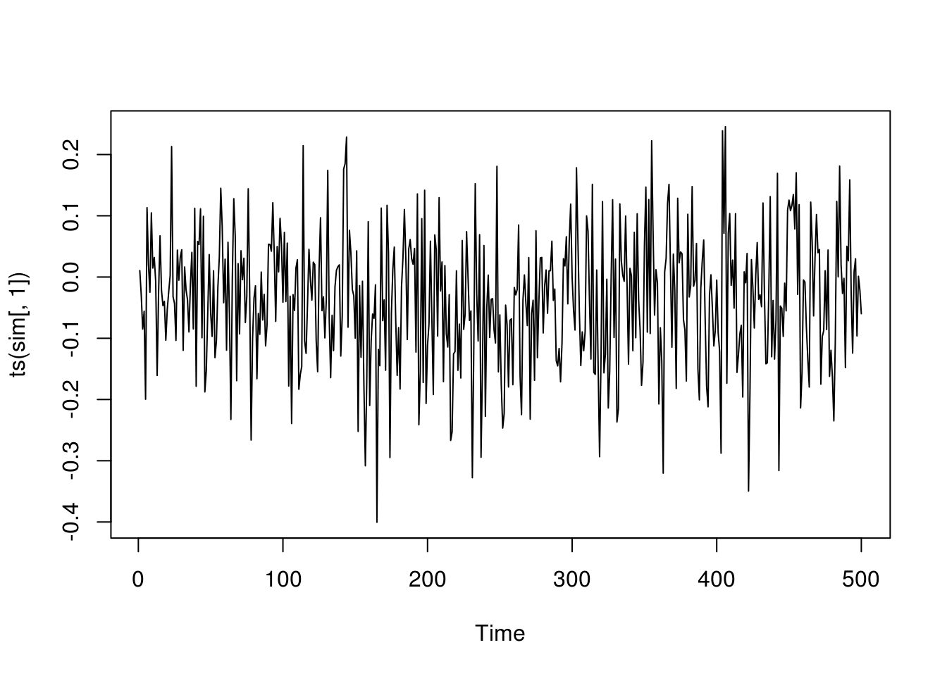

plot(ts(sim[,2]))

6.3 Exercises

6.3.1 Normal mixture revisited

Consider again the normal mixture example, except that the parameters of the normal distributions are considered unknown. Suppose that prior for \(\mu_1\) and \(\mu_2\) are \(N(0, 10^2)\), that the prior for \(1/\sigma_1^2\) and \(1/\sigma_2^2\) are \(\Gamma(a, b)\) with shape \(a = .5\) and scale \(b = 10\). Further, all the priors are independent. Design an MCMC using the Gibbs sampling approach to estimate all 5 parameters. You may use the arms()function in package HI. Run your chain for sufficiently long and drop the burn-in period. Plot the histogram of the results for all the parameters.

References

Robert, Christian, and George Casella. 2004. Monte Carlo Statistical Methods. Springer Science & Business Media.